Time Series Forecasting

A survey of statistical and deep learning models

What's a time series

A set of observations at regular time steps

from IPython.display import IFrame

# Source: https://data.gov.sg/dataset/hdb-resale-price-index
print("HDB Resale Price Index (Univariate)")
IFrame('https://data.gov.sg/dataset/hdb-resale-price-index/resource/52e93430-01b7-4de0-80df-bc83d0afed40/view/14c47d07-1395-4661-8466-728abce27f5f', width=600, height=400)

from IPython.display import IFrame

# Source: https://data.gov.sg/dataset/average-weekly-paid-hours-worked-per-employee-by-industry-and-type-of-employment-annual
print("Annual Average Weekly Paid Hours Worked Per Employee, By Industry And Type Of Employment (Multi-variate)")
IFrame('https://data.gov.sg/dataset/average-weekly-paid-hours-worked-per-employee-by-industry-and-type-of-employment-annual/resource/dd2147ce-20b7-401c-ac8f-8dbcc0d8e0d9/view/431f44b1-e58d-4131-998d-7e7aeee14479', width='600', height='400')

Time Series Introduction and Concepts

https://otexts.org/fpp2/intro.html

Time Series Decomposition

• For analysis
• Split into trend, cyclic, seasonal, noise
• Multiplicative or additive

Walkthrough: Time Series Decomposition

1. Go to https://data.gov.sg/dataset/hdb-resale-price-index
2. Click on the Download button
3. Unzip and extract the .csv file. Note that path to that file for use later.

We will use the StatsModels Python library to perform the decomposition.

This library will also be used later to perform statistical analysis. Pandas is also useful for manipulating time series data.

(mldds03) pip install statsmodels

"""Walkthrough: Time Series Decomposition"""

#!pip install statsmodels
from statsmodels.tsa.seasonal import seasonal_decompose
from matplotlib import pyplot as plt
import pandas as pd

# ==================================================================
# Dataset URL: https://data.gov.sg/dataset/hdb-resale-price-index
#
# Update this path to match your actual path
data_path = '../data/hdb-resale-price-index/housing-and-development-board-resale-price-index-1q2009-100-quarterly.csv'

# load data
df = pd.read_csv(data_path, index_col=0,
                 parse_dates=True, infer_datetime_format=True)

# print first few rows to make sure we loaded it properly
df.head(5)

DateTimeIndex

From the table above, we can confirm it is indeed a quarterly distribution.

seasonal_decompose (docs) expects a DateTimeIndex to indicate the frequency of the time series.

To enable this, we've set parse_dates=True and index_col=0 so that the DataFrame.index property is correctly set as a pandas.DatetimeIndex (docs), with a quarterly frequency.

# print the index.
# note that this is different from the "index" column in the DataFrame,
# which refers to the Resale Price Index.
print(df.index)

# plot the raw data, how that we have a DatetimeIndex
ax = df.plot()

Additive vs. Multiplicative Decomposition

Now we are ready to decompose. Let's try two models: additive and multiplicative.

You can find the definitions in the StatsModels documentation, but in a nutshell, the additive model "adds up" the components, while the multiplicative model "multiplies" the components together.

Additive: $$y(t) = Trend + Seasonal + Residual$$

Mulplicative: $$y(t) = Trend * Seasonal * Residual$$

# it's a bit confusing, but `index` here refers to the HDB resale price index,
# not the DataFrame.index (for time series)
additive = seasonal_decompose(df, model='additive')
additive.plot()
plt.show()

multiplicative = seasonal_decompose(df, model='multiplicative')
multiplicative.plot()
plt.show()

Observations

• There is a strong seasonal component. The component values are available as part of the object returned by seasonal_decompose
• The multiplicative model seems like a better fit, because the resulting residuals are smaller. In general, residuals (noise) are difficult to fit statistically.

Why decompose?

• The purpose of decomposition is to "subtract" known variability and simpilify creating models. For example, we can ignore the seasonal component and focus on predicting the trend.
• series_decompose uses a naive implementation. For a more advanced decomposition library, see STLDecompose

Frequency

https://github.com/statsmodels/statsmodels/blob/master/statsmodels/tsa/tsatools.py#L755

# print out the first few elements of each seasonal component
print('Multiplicative model: Seasonal component')
print(multiplicative.seasonal[:10])

print('Multiplicative model: Trend component')
print(multiplicative.trend[:10])

print('Additive model: Seasonal component')
print(additive.seasonal[:10])

print('Additive model: Trend component')
print(additive.trend[:10])

Forecasting

• Statistical: Auto-regressive, Moving average models

• Deep Learning: LSTMs

Auto-regressive models

$AR(p): X_t=c + \sum_{i=1}^p \varphi_iX_{t-i} + \varepsilon_t$

Output ($X_t$) depends on past values ($X_{t-i}$) + white noise ($\varepsilon_t$)

Fitting auto-regressive models

1. Use Autocorrelation to pick parameter $p$, which indicates how far back in time $X_{t-i}$ should go
2. Train model to fit data, minimizing mean squared error

Workshop: Auto-regressive Models

In this workshop, we'll take the dataset we've been working with and see if we can train an auto-regressive model for it.

Credits: borrowed heavily from https://machinelearningmastery.com/autoregression-models-time-series-forecasting-python/

"""Workshop: Auto-regressive Models"""

from matplotlib import pyplot as plt
import numpy as np
import pandas as pd
from statsmodels.tsa.seasonal import seasonal_decompose

# ==================================================================
# Dataset URL: https://data.gov.sg/dataset/hdb-resale-price-index
#
# Update this path to match your actual path
data_path = '../data/hdb-resale-price-index/housing-and-development-board-resale-price-index-1q2009-100-quarterly.csv'

# load data
df = pd.read_csv(data_path, index_col=0,
                 parse_dates=True, infer_datetime_format=True)

# print first few rows to make sure we loaded it properly
df.head(5)

Lag plots

A quick first test is to check if the data is random. If random, the data will not exhibit a structure in the lag plot.

Let's try pandas.plotting.lag_plot.

# try to see if there are correlations between X(t) and X(t-1)

fig, (ax1, ax2) = plt.subplots(nrows=2, ncols=1, figsize=(20,10))
df.plot(ax=ax1) # series plot
pd.plotting.lag_plot(df['index']) # lag plot

As a comparison, here's what the lag plot will look like for a random series:

# generate a random series
random_df = pd.DataFrame(np.random.randint(0, 100, size=(100, 1)))

fig, (ax1, ax2) = plt.subplots(nrows=2, ncols=1, figsize=(20,10))
random_df.plot(ax=ax1) # series plot
pd.plotting.lag_plot(random_df, ax=ax2) # lag plot (shows no correlation!)

So, it does look like there is correlation with the current and previous value of the HDB resale price index.

We are ready to move to the next step.

Auto-correlation plots

The next test is use auto-correlation to pick a good value of p to use for the equation:

$AR(p): X_t=c + \sum_{i=1}^p \varphi_iX_{t-i} + \varepsilon_t$

We will use the pandas.plotting.autocorrelation_plot: https://pandas.pydata.org/pandas-docs/stable/visualization.html#autocorrelation-plot

pd.plotting.autocorrelation_plot(df['index'])

Again, it is helpful to compare with a random series:

pd.plotting.autocorrelation_plot(random_df)

Interpreting Auto-correlation plots

The docs have a good explanation that we'll summarize here:

• Auto-correlation plots show the auto-correlation at different time lags (p)
• Random time series: the auto-correlations always hover around zero
• Non-random time series: find values of Lag where auto-correlations are outside of the 95% or 99% confidence band.
  • 95%: solid line
  • 99%: dashed line
• Both negative and positive auto-correlations are valid

Auto-regressive model

Since the dataset is about HDB quarterly resale prices, we can develop a model to predict the resale prices for the next year (4 quarters).

Recall that an Auto-regessive model uses the past values to predict the next value in the series:

$$AR(p): X_t=c + \sum_{i=1}^p \varphi_iX_{t-i} + \varepsilon_t$$

Baseline model

Before we fit the AR model, it's a good idea to create a baseline model.

The simplest possible one is a "Persistence Model", which just predicts the current value based on the last observation.

$$X_t = X_{t-1}$$

Predictions using a Persistence Model

1. The time series is a vector of (t, X) values. To model it, we will time-shift the dataset to produce two vectors (x, y).
   • input: $x = X_t$
   • output: $y = X_{t+1}$
2. We'll then split the (x, y) dataset into train and test

3. Run the baseline model to get predictions: $$\hat{y} = BaselineModel(x)$$ Where: $$BaselineModel(x) = x$$

4. Then compute the means square error: $$score = MSE(y, \hat{y})$$

def create_lagged_dataset(data):
    """Creates the dataset used for time-series modeling
    Args:
        data: the time series data (X)
    Returns:
        the lagged dataset (X[t], X[t+1]) as a pandas.DataFrame
    """
    values = pd.DataFrame(data)
    df = pd.concat([values.shift(1), values], axis=1) # concat in the column axis
    df.columns = ['t', 't+1']
    return df
    
def split_train_test(data, split_percent=10):
    """Splits the dataset into train and test sets
    Note that for time series data, we should not use random split
    because sequence is important.
    We'll just split by taking the last split_percent values
    
    Args:
        data: the dataset (x, y)
        split_percent: the percentage of the dataset to reserve
                       for testing
    Returns:
        tuple: (train, test) as pandas.DataFrames
    """
    split_index = int(((1-split_percent)/100) * data.shape[0])
    
    x = data.values
    train, test = x[1:split_index], x[split_index:]
    
    train_df = pd.DataFrame.from_records(train, columns=['x', 'y'])
    test_df = pd.DataFrame.from_records(test, columns=['x', 'y'])

    return train_df, test_df

def baseline_model(x):
    """Baseline model which gives the provided value
    It implements: f(x) = x
    Args:
        x: the value
    Returns:
        the provided value
    """
    return x

from sklearn.metrics import mean_squared_error

# create datasets
dataset = create_lagged_dataset(df['index'])
print("\nDataset:\n", dataset.head(5))

train, test = split_train_test(dataset)
print("\nTrain:\n", train.head(5))
print("\nTest:\n", test.head(5))

# walk-forward validation using baseline model: f(x) = x
baseline_predictions = [baseline_model(x) for x in test['x']]

# plot the predictions vs truth
_, ax = plt.subplots(figsize=(20,10))
f1, = ax.plot(test['y'])
f2, = ax.plot(baseline_predictions, color='red')
ax.legend([f1, f2], ['truth', 'baseline prediction'])
plt.show()

score = mean_squared_error(test['y'], baseline_predictions)
print("MSE:", score)

Auto-regressive model

Now that we have our baseline model in place, we can proceed with the AR model.

We'll use the statsmodels.tsa.ar_model.AR

Unlike the baseline model where we have to create a lagged time series, the AR model takes in a time series directly.

def split_train_test_timeseries(timeseries, split_percent=10):
    """Splits a time series DataFrame into train and test sets
    Note that for time series data, we should not use random split
    because sequence is important.
    We'll just split by taking the last split_percent values
    
    Args:
        timeseries: the time series DataFrame (index=date_time, X)
        split_percent: the percentage of the time series to reserve
                       for testing
    Returns:
        tuple: (train, test) as pandas.DataFrames
    """
    split_index = int(((1-split_percent)/100) * timeseries.shape[0])
    
    train = timeseries.iloc[:split_index, :]
    test = timeseries.iloc[split_index:, :]
    
    return train, test

from statsmodels.tsa.ar_model import AR

# create the Auto-regressive model using the training set
train_ts, test_ts = split_train_test_timeseries(df)
print("\nTrain:\n", train_ts.head(5))
print("\nTest:\n", test_ts.head(5))

model = AR(train_ts)

# fit the model
%time ar_model = model.fit()

print('Best lag: %s' % ar_model.k_ar)
print('Coefficients: %s' % ar_model.params)

The statsmodels.tsa.ar_model.AR implementation picked the 12-lag model as the best one.

Next, we'll make some predictions using the AR model.

test_start = pd.to_datetime(test_ts.index.values[0])
print("Start date", test_start)
test_end = pd.to_datetime(test_ts.index.values[-1])
print("End date", test_end)

ar_predictions = ar_model.predict(start=test_start, end=test_end)
baseline_predictions_ts = pd.DataFrame({'index': baseline_predictions}, index=ar_predictions.index)

# plot the predictions vs truth
_, ax = plt.subplots(figsize=(20,10))
f3, = ax.plot(test_ts)
f4, = ax.plot(ar_predictions, color='red')
f5, = ax.plot(baseline_predictions_ts, color='black')
ax.legend([f3, f4, f5], ['truth', 'AR(12) prediction', 'baseline prediction'])
plt.show()

score_ts = mean_squared_error(test_ts, ar_predictions)
print("MSE (AR 12):", score_ts)
print("MSE (baseline):", score)

What happened?

The AR fitted model performed MUCH WORSE than the baseline model.

Can you think of reasons to explain this?

Hint: look at the series, and think about what we are trying to predict here.

Try Decomposition?

Let's see if decomposition can help us fit a better model.

We'll use the Multiplicative model, because it appears to result in a smaller random component.

# ==================================================================
# Exercise:
# 1. Use multiplicative decomposition to extract the trend
#    Hint: You'll need to drop the first 2 NaN values using iloc
#    Otherwise, you'll get "LinAlgError: SVD did not converge"
#
#       df_trend = multiplicative.trend.dropna()
#












# 2. Re-train the AR model
#    Hint: use split_train_test_timeseries like above.












# 3. Compare the performance with the other models
#    Hint: you should plot 4 lines
#            truth
#            baseline
#            AR on original series
#            AR on multiplicative trend (new model)
#          you should also compute the MSE for predictions from the new model
#

Moving Average Model

We spent some time looking and trying out an Auto-regressive (AR) model.

Next: Moving Average (MA) model, and the combination of both.

Moving Average Model

$MA(p): X_t=\mu + \varepsilon_t + \sum_{i=1}^p\theta_i\varepsilon_{t-i}$

Output hovers around an average ($\mu$) and depends on past $p$ values of white noise ($\varepsilon_{t-i}$).

Auto-regressive, Moving Average Model (ARMA)

This is a combination of AR + MA:

$ARMA(p, q): AR(p) + MA(q)$

$X_t=c + \varepsilon_t + \sum_{i=1}^p \varphi_i X_{t-i} + \sum_{i=1}^q\theta_i\varepsilon_{t-i}$

Auto-regressive, Integrated Moving Average Model (ARIMA)

$ARIMA(p, d, q): \biggl(1-\sum_{i=1}^p\varphi_iB^i\biggr)(1 - B)^dX_t = c + \biggl(1 + \sum_{i=1}^q\theta_iB^i\biggr)\varepsilon_t$

(image: xkcd)

$ARIMA(p, d, q): X'_t = c + \varepsilon_t + \sum_{i=1}^p \varphi_i X'_{t-i} + \sum_{i=1}^q\theta_i\varepsilon_{t-i}$

$ARMA(p, d, q): X_t=c + \varepsilon_t + \sum_{i=1}^p \varphi_i X_{t-i} + \sum_{i=1}^q\theta_i\varepsilon_{t-i}$

$X'_t$ = $X_t$, Differentiated $d$ times

$X_t$ = $X'_t$, Integrated $d$ times (hence the I in ARIMA)

Think of ARIMA as something like:

1. $X' = Differential(X, degree=d)$
2. $X'_t = ARMA(X')$
3. $X_t = Integral(X'_t)$

Stationary Time Series

Mean, variance don't change over time (i.e. time-invariant)

Easier to model

Differentiation transforms a time series to become Stationary

Walkthrough: Time Series Stationarity

In this walkthrough, we will look at examples of stationary vs. non-stationary time series.

We'll also try modeling a non-stationary series using the ARIMA algorithm to see the effects of differentiation.

"""Walkthrough: Time Series Stationarity"""

from matplotlib import pyplot as plt
import numpy as np
import pandas as pd
from statsmodels.tsa.seasonal import seasonal_decompose

# ==================================================================
# Dataset URL: https://data.gov.sg/dataset/hdb-resale-price-index
#
# Update this path to match your actual path
data_path = '../data/hdb-resale-price-index/housing-and-development-board-resale-price-index-1q2009-100-quarterly.csv'

# load data
df = pd.read_csv(data_path, index_col=0,
                 parse_dates=True, infer_datetime_format=True)

# Plot a histogram of the observations
df.hist()

From the above histogram, this suggests a non-stationary series, where the mean and variance changes over time.

Let's plot histograms of the components.

multiplicative = seasonal_decompose(df, model='multiplicative')

# The seasonal component hovers around 3 values, and is stationary (time invariant)
multiplicative.seasonal.hist()

# The noise component is fairly gaussian and stationary (time invariant)
multiplicative.resid.hist()

# The trend changes with time, it's not stationary
multiplicative.trend.hist()

ARMA vs. ARIMA

Since the trend looks fairly non-stationary, let's explore predictions from both the Auto-regressive Moving Average (ARMA) and the Auto-regressive Integrated Moving Average (ARIMA) models.

This should also tell us if differentiation makes any difference in finding a stationary series that we can model.

ARMA: selecting best order

We will use Akaike's Information Criterion (AIC) and the Bayesian Information Criterion (BIC) to select the order.

More information about these metrics are at: www.otexts.org/fpp/8/6

In general, the smaller the better.

from statsmodels.tsa.arima_model import ARMA, ARIMA
from statsmodels.tsa.stattools import arma_order_select_ic

# We'll model the multiplicative trend
mult = seasonal_decompose(df, model='multiplicative')
trend = mult.trend.dropna()

# http://www.statsmodels.org/dev/_modules/statsmodels/tsa/stattools.html#arma_order_select_ic
# 'c' means constant
train_ts, test_ts = split_train_test_timeseries(trend)
res = arma_order_select_ic(train_ts, ic=['aic', 'bic'], trend='c')
print("Order that minimizes AIC:", res.aic_min_order)
print("Order that minimizes BIC:", res.bic_min_order)

Using the order ($p = 4, q = 2$) we will now fit the ARMA model.

# fit the model
order = res.aic_min_order
model = ARMA(train_ts, order)
%time arma_model = model.fit()
print("AIC:", arma_model.aic, "BIC:", arma_model.bic)

The AIC and BIC criteria are still quite large. This means that the model may not fit very well.

Let's give it a try anyway.

test_start = pd.to_datetime(test_ts.index.values[0])
test_end = pd.to_datetime(test_ts.index.values[-1])

# plot the forecast
_, ax = plt.subplots(figsize=(20, 10))
ax.plot(trend)
arma_model.plot_predict(start=test_start, end=test_end, dynamic=True, ax=ax)
plt.show()

# compute the MSE
predictions = arma_model.predict(start=test_start, end=test_end)
score = mean_squared_error(test_ts, predictions)
print("MSE (ARMA{}):".format(order), score)

The MSE is still significant, but much better than the AR model we looked at earlier.

Still not as good as the baseline though.

ARIMA

Finally, let's see what ARIMA can do. We'll use pyramid, which provides an order selector for ARIMA.

#!pip install pyramid-arima

from pyramid.arima import auto_arima

# auto_arima is a wrapper around R's auto.arima
# https://www.rdocumentation.org/packages/forecast/versions/7.3/topics/auto.arima
stepwise_fit = auto_arima(y=train_ts, start_p=1, start_q=1, max_p=10, max_q=10,
                          seasonal=True, max_d=5, trace=True,
                          error_action='ignore', # don't want to know if an order does not work
                          suppress_warnings=True, # don't want convergence warnings
                          stepwise=True)  # set to stepwise

stepwise_fit.summary()

The best fit appears to be with $p = 2, d = 1, q = 1$

order_arima = (2, 1, 1)
model = ARIMA(train_ts, order_arima)
%time arima_model = model.fit()
print("AIC:", arima_model.aic, "BIC:", arima_model.bic)

Better AIC and BIC than the ARMA model.

test_start = pd.to_datetime(test_ts.index.values[0])
test_end = pd.to_datetime(test_ts.index.values[-1])

# plot the forecast
_, ax = plt.subplots(figsize=(20, 10))
ax.plot(trend)
arima_model.plot_predict(start=test_start, end=test_end, dynamic=True, ax=ax)
plt.show()

# compute the MSE
predictions = arima_model.predict(start=test_start, end=test_end, typ='levels')

score = mean_squared_error(test_ts, predictions)
print("MSE (ARMA{}):".format(order), score)

Further Reading

Additional topics that are not covered, but worth reading up on:

• Vector Auto-regressive model (VAR) for multi-variate time series
• Partial auto-correlation plots
• Seasonal ARIMA (SARIMA)
• ARIMA with eXogeneous variables (ARIMAX)
• SARIMAX (basically a combo of the above two)

statsmodels:

• SARIMAX, covers SARIMA, ARIMAX, and SARIMAX
• VAR
• Partial Auto-correlation plots

Deep Learning models for Time Series

Limitations of Statistical Models

• need to pick order
• sometimes won't converge
• complex to model non-linearity

Recurrent Networks for Time Series

• LSTM unit + Fully Connected
  • Train with enough data
  • Profit!
• Stack more LSTMs for more complicated series (e.g. multi-variate)
• GRU? Why not!

Walkthough: RNN Time Series Predictor

Dataset: Average Weekly Paid Hours Worked Per Employee By Industry And Type Of Employment, Annual

Link: https://data.gov.sg/dataset/average-weekly-paid-hours-worked-per-employee-by-industry-and-type-of-employment-annual?resource_id=ecc88c54-6d33-4d1c-9af5-896825386d56

Download, unzip, and note the path and replace it below.

Credits: https://machinelearningmastery.com/time-series-forecasting-long-short-term-memory-network-python/

Cheatsheets:

• https://s3.amazonaws.com/assets.datacamp.com/blog_assets/PandasPythonForDataScience.pdf
• https://s3.amazonaws.com/assets.datacamp.com/blog_assets/Python_Matplotlib_Cheat_Sheet.pdf

"""Walkthrough: RNN Time Series Predictor"""

import numpy as np
import pandas as pd
from matplotlib import pyplot as plt

# ==================================================================
# Dataset URL: https://data.gov.sg/dataset/average-weekly-paid-hours-worked-per-employee-by-industry-and-type-of-employment-annual
#
# Update this path to match your actual path
data_path = '../data/weekly-paid-hours/average-weekly-paid-hours-worked-per-employee-by-type-of-employment-topline.csv'

# load data
df = pd.read_csv(data_path, index_col=0,
                 parse_dates=True, infer_datetime_format=True)

# Inspect
df.tail(5)

# let's filter by full-time vs. part-time when we plot
df_ft = df[df['nature_of_employment'] == 'full-time']
df_pt = df[df['nature_of_employment'] == 'part-time']

_, ax = plt.subplots(nrows=1, ncols=1, figsize=(20, 10))
df_ft.plot(ax=ax, marker='o')
df_pt.plot(ax=ax, marker='x')

Prediction Task

Let's define our prediction task.

• Task: Predict the Full Time, Total Paid Hours for 2018-2020
• Training set: Annual data for 1990-2011
• Test set: Annual data for 2012-2016
• Model: RNN with single LSTM layer
• Baseline model: persistence model

Baseline model

All performance is relative. First, let's run the baseline model so that we have something to compare the performance of RNN.

def get_split_row_index(data, split_date_str):
    """Gets the split index for the data, given a date string
    Args:
        data: the dataframe containing (t, X)
        split_date_str: a date string format that's acceptable by
                        pandas.to_datetime()
    Returns:
        the split row index into data
    """
    split_date = pd.to_datetime(split_date_str)
    split_data = data[data.index <= split_date]
    return split_data.shape[0]

def create_lagged_dataset(data):
    """Creates the dataset used for time-series modeling
    Args:
        data: the dataframe containing (t, X)
    Returns:
        the lagged dataset (X[t], X[t+1]) as a pandas.DataFrame
    """
    values_df = pd.DataFrame(data.values)
    df = pd.concat([values_df.shift(1), values_df],
                   axis=1) # concat in the column axis
    df.columns = ['t', 't+1']
    return df.dropna()

def create_train_test(data, split_date_str):
    """Splits the dataset into train and test sets
    Note that for time series data, we should not use random split
    because sequence is important.
    We'll just split by reserving the values after the split_date
    into the test set.
    
    Args:
        data: the dataframe containing (t, X)
        split_date_str: entries after this date string will be
                        reserved in the test set. This should be
                        a string format that's acceptable by
                        pandas.to_datetime()
    Returns:
        tuple: (train, test) as pandas.DataFrames
    """
    # first, convert the split date into a split index
    split_index = get_split_row_index(data, split_date_str)
    
    # next, create the lagged dataset (X[t], X[t+1])
    lagged_dataset = create_lagged_dataset(data['total_paid_hours'])

    # finally, split the lagged dataset using the split index
    train = lagged_dataset[:split_index]
    test = lagged_dataset[split_index:]
    return train, test

def baseline_model(x):
    """Baseline model which gives the provided value
    It implements: f(x) = x
    Args:
        x: the value
    Returns:
        the provided value
    """
    return x

from sklearn.metrics import mean_squared_error

# use only the columns we care about
df_ft = pd.DataFrame(df[df['nature_of_employment'] == 'full-time'],
                     columns=['total_paid_hours'])

train, test = create_train_test(df_ft, '2012')

print("\nTrain dataset:\n", train.head(5))
print("\nTest dataset:\n", test.head(5))

# walk-forward validation using baseline model: f(x) = x
baseline_predictions = [baseline_model(x) for x in test['t']]
print("\nPredictions:\n", baseline_predictions)

# plot the predictions vs truth
_, ax = plt.subplots(figsize=(20,10))
f1, = ax.plot(test['t+1'].values, marker='o')
f2, = ax.plot(baseline_predictions, color='red', marker='o')
ax.legend([f1, f2], ['truth', 'baseline prediction'])
plt.show()

score = mean_squared_error(test['t+1'], baseline_predictions)
print("MSE:", score)

LSTM RNN

Now we are ready to train our RNN to see if it can beat the baseline model.

We will keep the architecture simple and create a single-layer LSTM that feeds into a fully-connected (Dense) layer.

model = Sequential()
model.add(LSTM(...))
model.add(Dense(1))
model.compile(loss='mean_squared_error', optimizer='adam')

Note: As an exercise, you are encouraged to try the Statistical models as well.

RNN: preparing data

Convert to Supervised dataset

Unlike statistical models, RNN is a supervised learning problem. This means that we'll need to convert the data from a time series $(t, X)$ to a supervised learning dataset $(x, y)$.

Because the baseline model is also a supervised learning problem, we can reuse create_train_test as long as we keep the inputs and outputs in the same data type (e.g. pandas.DataFrame, same column names...).

Differencing

To improve the modeling, we'll try to remove non-stationarity from the data. We'll use a technique called "differencing," where computing the change in value for each time step, relative to the previous time step.

def difference(series):
    """Computes the difference of a series,
    which contains the relative change in value from
    the previous entry
    Args:
        series: the series
    Returns:
        the differenced values (change relative
        to the previous step)
    """
    values = series.values
    diff = [values[i] - values[i - 1]
            for i in range(1, len(values))]
    return pd.DataFrame(diff)

def inverse_difference(initial_value, differenced):
    """Computes the inverse difference of a series
    Args:
        initial_value: the initial value
        differenced: the differenced series as a
                     panda.DataFrame
    Returns:
        the original series as a panda.DataFrame
    """
    diff = differenced.values

    data = np.ndarray(differenced.shape[0] + 1)
    data[0] = initial_value

    for i in range(len(diff)):
        data[i+1] = data[i] + diff[i]
    return pd.DataFrame(data)

def difference_unittest():
    series = pd.DataFrame([1., -2., 3., -4., 5.])
    d = difference(series)
    s = inverse_difference(series[0][0], d)
    np.testing.assert_allclose(series.values, s.values)

difference_unittest()

Scaling

LSTMs use tanh activations, so we will need to scale the data to -1 and 1.

We'll use the training dataset to scale the data, so that there is no contamination from the test dataset.

from sklearn.preprocessing import MinMaxScaler

def scale(train, test, scale_range=(-1, 1)):
    """Scales data to the feature_range
    Args:
        train: the training set
        test: the test set
        scale_range: the range (inclusive) to scale
    Returns:
        a tuple of scaler, scaled_train, scaled_test data
    """
    scaler = MinMaxScaler(feature_range=scale_range)
    scaler = scaler.fit(train)

    # sanity check, print the min, max observed by the scaler
    print("Training min:", scaler.data_min_,
          "Training max:", scaler.data_max_)

    train_scaled = scaler.transform(train)

    # test dataset uses a scaler fit to the min & max of training set
    test_scaled = scaler.transform(test)

    return scaler, train_scaled, test_scaled

def inverse_scale(scaler, scaled_data):
    """Restores the data back to the original scale
    Args:
        scaler: the scaler, used to scale the original data
        scaled_data: the data to unscale
    Returns:
        the unscaled data        
    """
    return scaler.inverse_transform(scaled_data)

def scale_unittest():
    train = pd.DataFrame([10., -2., 30., -4., 5.])
    test = pd.DataFrame([1., -2., 3., -4., 50.])
    scaler, train_scaled, test_scaled = scale(train, test)
    test_unscaled = inverse_scale(scaler, test_scaled)
    np.testing.assert_allclose(test.values, test_unscaled)
    
scale_unittest()

Putting it together: Data Processing

We'll now do the following:

1. Compute the differenced series for full-time, total_paid_hours
2. Scale the dataset based on the training set's max and min
3. Convert the series into a supervised dataset, split into train and test

# Starting point DataFrame
df_ft = pd.DataFrame(df[df['nature_of_employment'] == 'full-time'],
                     columns=['total_paid_hours'])

df_ft.head(5)

# Step 1: Compute the difference

df_ft_diff = difference(df_ft['total_paid_hours'])
df_ft_diff.index = df_ft.index[1:]
df_ft_diff.columns = ['total_paid_hours']

df_ft_diff.head(5)

# Step 2: Scale the dataset for training with LSTM
split_index = get_split_row_index(df_ft_diff, "2012")
df_train, df_test = df_ft_diff[:split_index], df_ft_diff[split_index:]

scaler, train_scaled, test_scaled = scale(df_train.values, df_test.values)
print("Train scaled:")
print(train_scaled[:5])

print("Test scaled:")
print(test_scaled[:5])

# Step 3: Convert to a supervised learning datasets
train = create_lagged_dataset(pd.DataFrame(train_scaled))
test = create_lagged_dataset(pd.DataFrame(test_scaled))
train.head(5)

test.head(5)

Differencing makes a ... difference

Since we are scaling the test dataset based on the training dataset, it is possible for the test truth values to fall completely outside of the [-1, 1] range.

Truth values outside of the range will mean higher mean squared error with the RNN model. We would encounter this if we did not apply differencing to the series, because the test truth values were lower than the training values.

In general, whenever you observe a time-dependent trend in the data, it is a good idea to try differencing as a pre-processing step.

Optional Exercise - Differencing with Auto Regression

Differencing can be helpful for modeling the HDB Resale Price dataset. Try it before feeding into the Statistical models to see if you get better predictions.

Setting up the LSTM RNN

Using Keras, we'll now setup an LSTM Recurrent Neural Network with the this configuration:

• Neurons (how many LSTM units): 1
• Loss: mean square error
• Optimizer: Adam
• Input shape: batch size, # time steps, # features
  • batch size: 1
  • time steps: 1
  • features: 1

from keras.models import Sequential
from keras.layers import Dense, LSTM

def create_LSTM_model(batch_size, time_steps, features, neurons):
    """Creates the LSTM model for predicting time-series
    Args:
        batch_size: number of samples per batch
        time_steps: number of time steps per sample
        features: number of features per sample
        neurons: number of LSTM neurons
    Returns:
        the model
    """
    model = Sequential()
    model.add(LSTM(neurons,
                   batch_input_shape=(batch_size, time_steps, features), 
                   stateful=True))
    model.add(Dense(1))
    model.compile(loss='mean_squared_error', optimizer='adam')
    return model

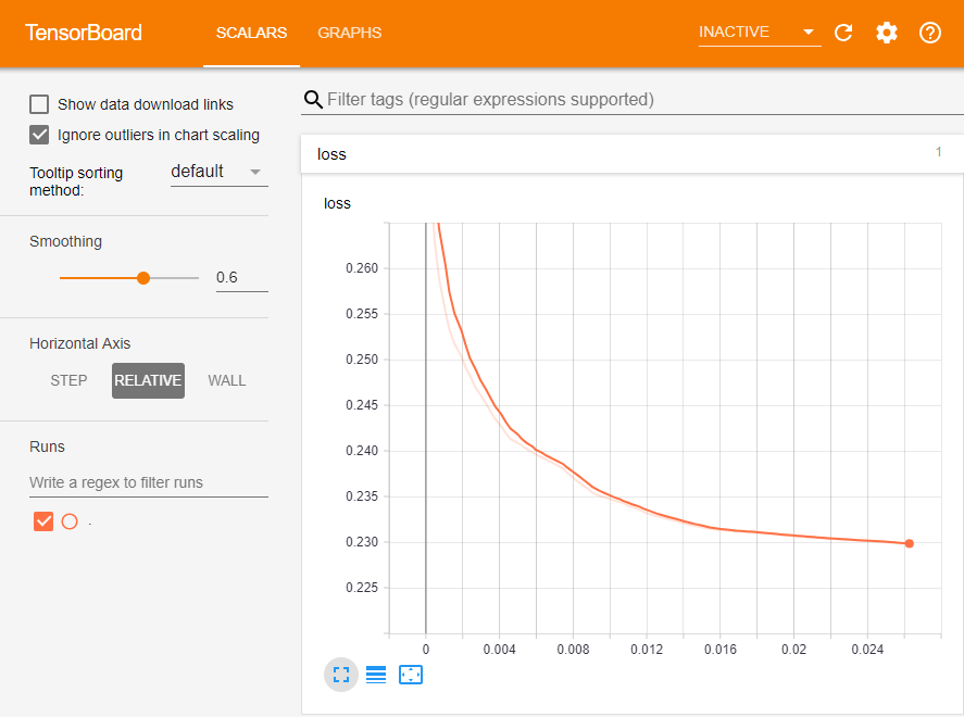
TensorBoard Callbacks

Because the model is being re-fit on each epoch, we'll extend the Keras Tensorboard callback to log the losses for each epoch.

This way we can visualize the losses.

from keras.callbacks import TensorBoard
import tensorflow as tf
from time import time

class LossHistory(TensorBoard):
    writer = None
    log_dir = None

    def __init(self, log_dir='./logs', **kwargs):
        """Constructor
        Args:
            log_dir: the logs directory
        """
        # make a subdirectory for our loss logs
        self.log_dir = os.path.join(log_dir, 'loss')
        super(LossHistory, self).__init__(log_dir, **kwargs)

    def set_model(self, model):
        """Called by Keras to set the model
        Args:
            model: the model being set
        """
        # setup the writer for the loss metric
        self.writer = tf.summary.FileWriter(self.log_dir)
        super(LossHistory, self).set_model(model)

    def on_epoch_end(self, epoch, logs={}):
        """Called by Keras during the end of an epoch
        Args:
            epoch: the current epoch
            logs: the statistics to be logged
        """
        # record the loss in the summary so that
        # TensorBoard will plot it
        summary = tf.Summary()
        summary_value = summary.value.add()
        summary_value.simple_value = logs.get('loss')
        summary_value.tag = 'loss'
        self.writer.add_summary(summary, epoch)
        self.writer.flush()
        super(LossHistory, self).on_epoch_end(logs, epoch)

Training

We'll now train the RNN.

If all goes well, you should see a loss curve like this in TensorBoard:

# Model configuration
NEURONS = 1
TIME_STEPS = 1
BATCH_SIZE = 1
EPOCHS=3000
FEATURES=1

X_train = train['t']
y_train = train['t+1']

# reshape the data to (samples, timesteps, features)
X_train = X_train.reshape(len(X_train), TIME_STEPS, FEATURES)
print("(samples, timesteps, features):", X_train.shape)

# setup logging
tensorboard = LossHistory(log_dir='./logs/lstm_ts_{}'.format(time()),
                          write_graph=True, write_images=True)

# create the model
model = create_LSTM_model(batch_size=BATCH_SIZE, time_steps=TIME_STEPS,
                          features=FEATURES, neurons=NEURONS)

# train
for i in range(EPOCHS):
    # IMPORTANT: shuffle must be False because
    # ordering of samples needs to be preserved and learnt
    model.fit(X_train, y_train, epochs=1, batch_size=BATCH_SIZE,
              verbose=True, shuffle=False, callbacks=[tensorboard])
    
    # Reset the state for each epoch because we are starting
    # from the beginning of the sample
    # This does not reset the weights, just the hidden states
    model.reset_states()

Making Predictions

After training the LSTM, we can use it to make predictions:

1. Initialize the state in the network using the training data
2. Make the prediction for each test data
3. Invert scaling
4. Invert differencing
5. Plot and compute mean square error

def initialize_model_state(model, train):
    """Initializes the model state using training data
    Args:
        model: the trained model
        train: the training set use
    Returns:
        the initialized model
    """
    # "fast forward" the model to the end of the
    # training timesteps (X_train), discarding the
    # predictions (yhat_train)
    X_train = train['t']
    
    # reshape to samples, time steps, features
    X_train = X_train.reshape(len(X_train), 1, 1)
    
    # predict with batch_size=1 to
    # initialize the model to the last value of
    # of the training set
    model.predict(X_train, batch_size=1)

def one_step_forecast(model, batch_size, X):
    """Makes a single-step forecast
    Args:
        model: the trained model
        batch_size: the batch size
        X: input for the next step as a numpy.ndarray
    Returns:
        forecast for the next step as a scalar
    """
    # reshape to samples, time steps, features
    X = X.reshape(1, 1, 1)
    yhat = model.predict(X, batch_size=batch_size)
    return yhat[0, 0]

test_values = test['t'].values

# make predictions as a column list of lists, to
# match how the original scaler is fitted
predictions = [[one_step_forecast(model, 1, test_values[i])] 
               for i in range(len(test_values))]

# invert scaling
predictions = inverse_scale(scaler, predictions)

# invert differencing
last_training_sample = df_ft.values[split_index-1]
predictions = inverse_difference(last_training_sample,
                                 pd.DataFrame(predictions))

# shift predictions to exclude the last_training_sample
# which was only used for inverting the differencing
rnn_predictions = predictions.values[1:]
print("RNN predictions:", rnn_predictions)

# plot the predictions vs baseline vs truth
_, ax = plt.subplots(figsize=(20,10))

_, truth = create_train_test(df_ft, "2012")
truth_values = truth['t+1'].values
f1, = ax.plot(truth_values, marker='o')
f2, = ax.plot(baseline_predictions, color='red', marker='o')
f3, = ax.plot(rnn_predictions, color='black', marker='o')
ax.legend([f1, f2, f3], ['truth', 'baseline prediction', 'RNN prediction'])
plt.show()

score_rnn = mean_squared_error(truth_values, rnn_predictions)
print("RNN MSE:", score_rnn)

score_baseline = mean_squared_error(truth_values, baseline_predictions)
print("Baseline MSE:", score_baseline)

Exercise: Forecasting

Assuming the RNN can be tuned to be sufficiently accurate, we can also use it to predict future readings.

This is one advantage it offers over the baseline model, which will not be as useful for forecasting after time_step+1.

# ==========================================================
# Exercise: use the RNN to predict the next 3 years (2018-2020)
# and plot the forecasted values
#
# Hint: use np.asarray to convert a single prediction 'row'
#       entry to a numpy array

# predict based on original test values (up to 2017)
predictions = [[one_step_forecast(model, 1, test_values[i])] 
               for i in range(len(test_values))]

# Your code here












# plot the predictions vs baseline vs truth
_, ax = plt.subplots(figsize=(20,10))

f1, = ax.plot(truth_values, marker='o')
f2, = ax.plot(baseline_predictions, color='red', marker='o')
f3, = ax.plot(rnn_predictions, color='green', marker='o')
ax.legend([f1, f2, f3],
          ['truth', 'baseline prediction', 'RNN forecast'])

plt.show()

Practice Exercises:

1. Try tuning the hyperparameters for the LSTM network to improve its score: more epochs, more neurons
2. Try a GRU instead of LSTM, and compare the results
3. Skip differencing to see what the effect is on accuracy
4. Try using your own time series dataset. This is good practice for data processing and problem definition.

When doing these exercises, practice using TensorBoard and the score to evaluate the difference in performance. Which method will you recommend most?

Further Reading

• Engineering Extreme Event Forecasting at Uber with Recurrent Neural Networks
• Instability of Online Learning for Stateful LSTM for Time Series Forecasting