Speech Recognition
A survey of statistical and deep learning models
Automatic Speech Recognition Pipeline

(image: https://www.techrepublic.com/article/how-we-learned-to-talk-to-computers/)
Terminology
Phoneme: basic unit of sound (e.g. /e/ in 'pet')
Grapheme: letter(s) that represent phonemes (e.g. sh, ng)
Acoustic model: maps audio signals to phonetic units (phonemes or graphemes)
Language model: maps phonetic units to word sequences
Utterance: spoken input (word, phrase, sentences)
Terminology
Speaker-dependent speech recognition: recognizes only users it is trained for. Usually large vocabulary but few speakers.
Speaker-independent speech recognition: recognizes multiple users without training. Usually small vocabulary.
Word Error Rate
$WER = \frac{S + D + I}{N}$
- substitution word count: $S$
- deletion word count: $D$
- insertion word count: $I$
- correct word count: $C$
- number of reference words: $N = S + D + C$
Sometimes called the "Length Normalized Edit Distance"
Word Accuracy
$WAcc = 1 - WER = \frac{(N - S - D) - I}{N} = \frac{C - I}{N}$
Speech Feature Extraction
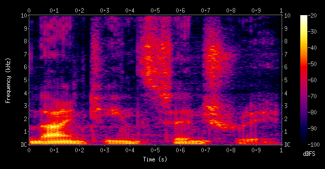 (Image: Wikipedia)
A spectrogram for "nineteen century" - power vs. frequency
Common method: Mel-frequency cepstral coefficients (MFCC)
Statistical Speech Recognition
$$W^* = \underset{W}{\operatorname{argmax}}P(W \mid X)$$
- word sequence: $W$
- most likely word sequence: $W^*$
- acoustic input feature vector (e.g. MFCC): $X$
Statistical Speech Recognition
After Bayes' Theorem:
$$W^* = \underset{W}{\operatorname{argmax}}p(X \mid W)P(W)$$
- acoustic model: $p(X \mid W)$
- language model (e.g. N-gram): $P(W)$
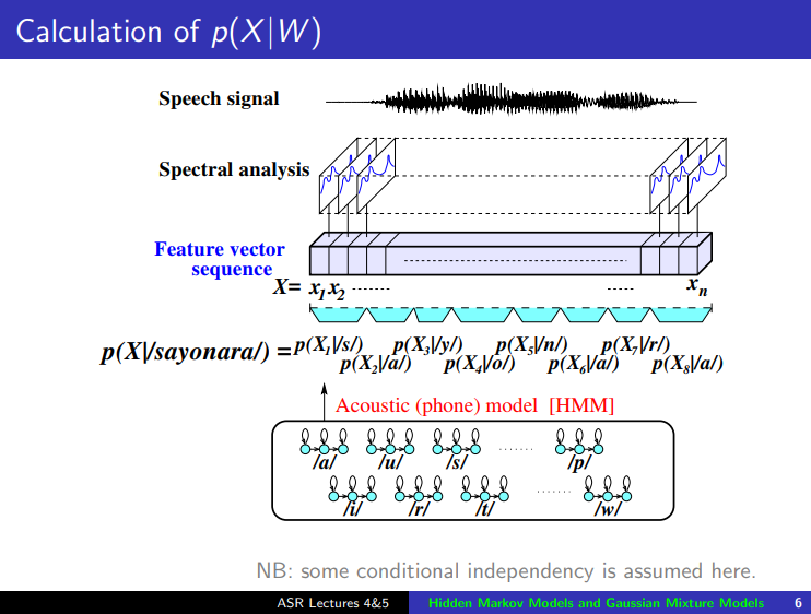
Statistical Acoustic Model: $p(X|W)$
(image: https://www.inf.ed.ac.uk/teaching/courses/asr/2016-17/asr03-hmmgmm-handout.pdf)
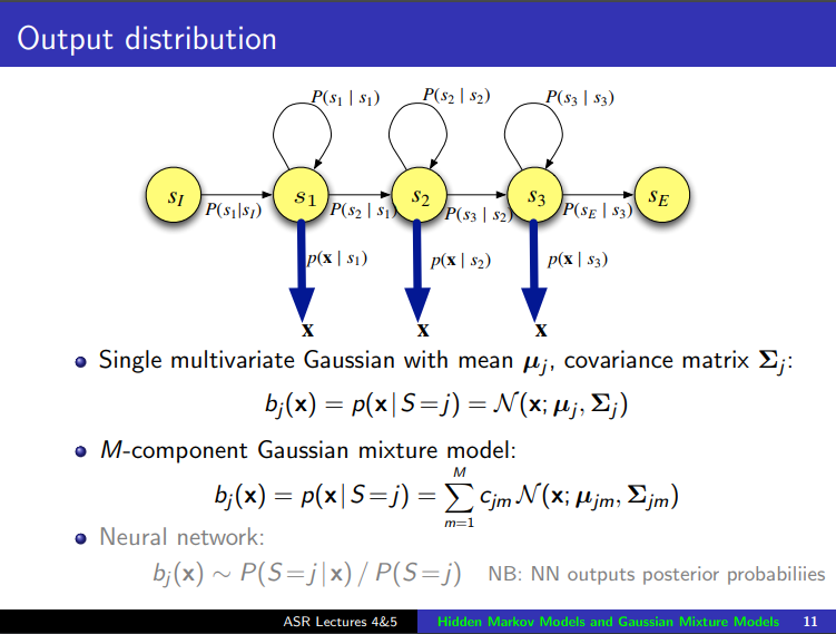
Hidden Markov Model: $p(S_i \mid S_{i-1})$, Gaussian Mixture Model: $p(X \mid S_i)$
(image: https://www.inf.ed.ac.uk/teaching/courses/asr/2016-17/asr03-hmmgmm-handout.pdf)
Gaussian Mixture Model
Mixture distribution: combine multiple probabability distributions to make an improved model
$$P(x) = \sum_iP(c=i)P(x \mid c=i)$$
$i^{th}$ Gaussian component: $P(x \mid c=i)$
Applications
- Clustering
- Classification
Nice intro: https://yulearning.blogspot.sg/2014/11/einsteins-most-famous-equation-is-emc2.html
Workshop: GMM gender detector
Credits: https://github.com/abhijeet3922/PyGender-Voice
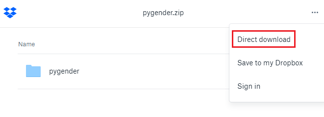
Download data from here
Extract the .zip file to a folder of your choice. Note down the path as you will need to enter it in the workshop code.
import os
from os.path import basename, join
import numpy as np

from python_speech_features import mfcc
from scipy.io.wavfile import read
from sklearn import preprocessing
from sklearn.mixture import GaussianMixture

TRAIN_PATH = 'C:\\mldds\\pygender\\train_data\\youtube\\' # modify to your actual path
def get_MFCC(audio_file, scale=True):
    """Computes the Mel-frequency ceptrum coefficients for an audio file
    Args:
        audio_file: input audio file
        scale: whether to scale the features between 0-1
    Returns:
        the MFCC features
    """
    sample_rate, audio = read(audio_file)
    features = mfcc(audio, sample_rate, winlen=0.025, winstep=0.01,
                    numcep=13, appendEnergy=False)
    if scale:
        features = preprocessing.scale(features) # scale to (0, 1)
    return features
# Playback a sample file
from IPython import display

sample_file = join(TRAIN_PATH, 'male', 'male1.wav')
sample_rate, audio = read(sample_file)
display.Audio(data=audio, rate=sample_rate)
# Plot the MFCC
import matplotlib.pyplot as plt

mfcc_vector = get_MFCC(sample_file, scale=False)
fig, ax = plt.subplots(nrows=1, ncols=1, figsize=(20,4))
cax = ax.matshow(np.transpose(mfcc_vector), interpolation='nearest',
                 aspect='auto', cmap='plasma', origin='lower')
fig.colorbar(cax)
plt.title("Spectrogram of {}".format(sample_file))
plt.show()
def train_GMM(data_path, n_components=8, covariance_type='diag'):
    """Trains a Gaussian mixture model
    Args:
        data_path: data folder path
        n_components: number of Gaussian components
        covariance_type: type of covariance matrix
    Returns:
        the GMM model
    """
    files = [join(data_path, f) for f in os.listdir(data_path) if f.endswith('.wav')]
    features = np.asarray(());

    for f in files:
        mfcc_vector = get_MFCC(f)

        if features.size:
            features = np.vstack((features, mfcc_vector))
        else:
            features = mfcc_vector

    gmm = GaussianMixture(n_components=n_components,
                          covariance_type=covariance_type,
                          max_iter=200, n_init=3)
    gmm.fit(features)

    # print some metrics applicable to GMMs
    print('BIC: ', gmm.bic(features), ', AIC: ', gmm.aic(features))
    return gmm
models = dict()
%time models['male'] = train_GMM(join(TRAIN_PATH, 'male'), n_components=8, \
                                 covariance_type='diag')

# ==================================================================
# Exercise:
# Add code below to train the female model, using the above as an example


# ==================================================================
# Optional Exercises:
# a. Try different values of n_component (e.g. 2, 16)
# b. Try different values of covariance_type (e.g. full)
#
# See http://scikit-learn.org/stable/modules/generated/sklearn.mixture.GaussianMixture.html
# on how to interpret the BIC and AIC metrics for selecting models
def test_GMM(models, test_data_path):
    """Trains a Gaussian mixture model
    Args:
        models: {name: gmm} dictionary of models
        test_data_path: test data folder path
    Returns:
        the predictions
    """
    files = [os.path.join(test_data_path,f) for f in os.listdir(test_data_path)
             if f.endswith(".wav")]

    predictions = []
    for f in files:
        features = get_MFCC(f)
        keys = []
        log_likelihood = np.zeros(len(models))

        for i, (key, gmm) in enumerate(models.items()):
            scores = np.array(gmm.score(features))
            keys.append(key)
            log_likelihood[i] = scores.sum()

        # find the model with the maximum score
        winner = np.argmax(log_likelihood)
        # print('prediction:', keys[winner], "\tscores:", log_likelihood[winner])
        predictions.append(keys[winner])
    return predictions
# ==================================================================
# Exercise:
# 1. Complete the code below to test the GMM models using test_GMM().
#    Be sure to run against both male and female models.
# 2. Plot the confusion matrix

from sklearn.metrics import confusion_matrix

TEST_PATH = 'C:\\mldds\\pygender\\test_data\\AudioSet' # modify to your actual path
Shortcomings of Statistical Approaches
Lots of hand-tuning
Inefficient for approximating non-linear data: combination covariance matrices get very large / complicated
Solution: deep learning
Deep Belief Nets
- Replaces the Gaussian Mixture Model in an ASR system
- Generative pre-training
- Speeds up training with less overfitting
- Train a hidden layer (using Restricted Boltmann Machines or Gaussian RBM)
- Use the weights as inputs to train next layer
- Stack up into a forward-only "Deep Belief Net" (DBN)
- Add softmax to create the DBM-DNN
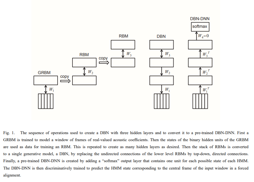
(image: Hinton et al.)
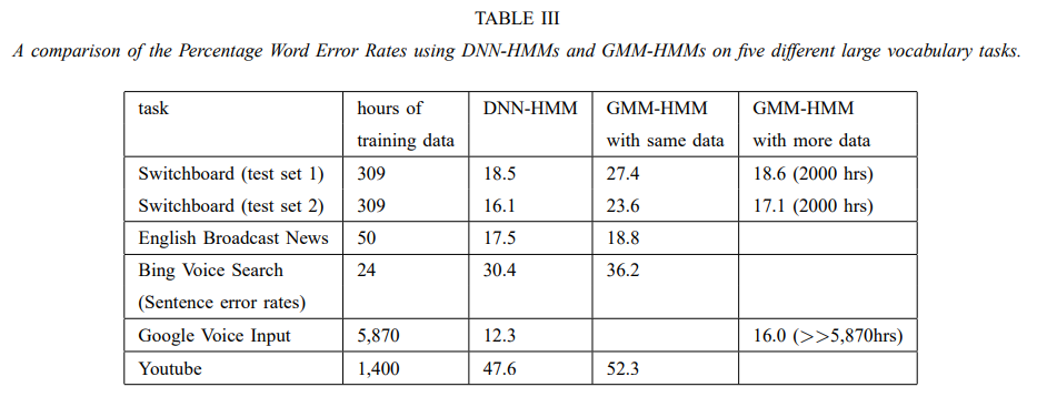
(image: Hinton et al.)
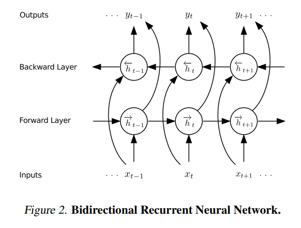
Birectional RNN
- Forward $$\overrightarrow{h}^l_t = g(h^{l-1}_t, \overrightarrow{h}^l_{t-1})$$
- Backward $$\overleftarrow{h}^l_t = g(h^{l-1}_t, \overleftarrow{h}^l_{t+1})$$
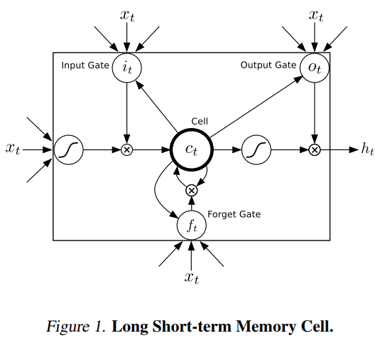
- $g(.)$ can be recurrent, GRU, LSTM
- Learns context in both directions (like words in speech)
Correctionist Temporal Classification
https://www.cs.toronto.edu/~graves/icml_2006.pdf
- Goal: a temporal classifier that can classify unseen audio input sequences with low error rate
- To train speech to text, we need to know how audio "lines up" with transcripts
- Input sequences: $X$ (such as audio)
- Output sequences: $Y$ (such as transcripts)
- Error rate: normalized edit distance between predicted and target labels
Problem: $X$ and $Y$ can vary in length, in different ways
Solution: introduce the blank token ($\epsilon$)
Process: train an RNN to estimate probabilities of each character per time step
(images: Hannun)
CTC implementation
- Recurrent neural network, e.g. bidirectional LSTM
- CTC loss function, maximize log likelihood
- Decoding: prefix search instead of best path search
(image: Visual Guide and Explanation)
Walkthrough: Correctionist Temporal Classification
"""This is a simple example that illustrates how CTC is computed from TensorFlow
For brevity, it only supports 1 training input and 1 validation input
For an example of batched input, use:
https://github.com/philipperemy/tensorflow-ctc-speech-recognition
"""

# !pip3 install jupyter-tensorboard

import os
import sys
import numpy as np
from os.path import join
from python_speech_features import mfcc
from scipy.io.wavfile import read
from sklearn import preprocessing
import tensorflow as tf
import time

# Constants
SPACE_TOKEN = '<space>'
SPACE_INDEX = 0
FIRST_INDEX = ord('a') - 1  # 0 is reserved to space

# Configuration
num_features = 13
num_units = 50 # Number of units in the LSTM cell

# Number of classes: 'a' to 'z' +  space + blank label = 28 characters
num_classes = ord('z') - ord('a') + 1 + 1 + 1

# Hyper-parameters
num_epochs = 200
num_hidden = 50
# Get training and validation inputs
num_layers = 1
batch_size = 1
initial_learning_rate = 1e-2
momentum = 0.9
# Get training and validation inputs
# Validation input is just the training audio shifted randomly

def process_audio(audio_file, do_random_shift=None):
    """Extracts the MFCC features from an audio file.
    Args:
        audio_file: file containing the input audio
        do_random_shift: whether to randomly shift the audio
                      (e.g. for generating test inputs)
    Returns:
        A tuple with (features, sequence length)
    """
    sample_rate, audio = read(audio_file)

    if do_random_shift:
        random_shift = np.random.randint(low=1, high=1000)
        print('random_shift =', random_shift)
        truncated_audio = audio[random_shift:]

    features = mfcc(audio, sample_rate)
    features = preprocessing.scale(features) # scale to (0, 1)

    features = np.asarray(features[np.newaxis, :])
    features_seq_len = [features.shape[1]]
    return features, features_seq_len

# audio_file = join('files', 'CTC', 'LDC93S1.wav')
audio_file = join('files', 'CTC', '61-70968-0002.wav')

train_input, train_seq_len = process_audio(audio_file)
val_input, val_seq_len = process_audio(audio_file, do_random_shift=True)
def sparse_tuple_from(sequences, dtype=np.int32):
    """Create a sparse representation of sequences.
    Args:
        sequences: a list of lists of type dtype where each element is a sequence
    Returns:
        A tuple with (indices, values, shape)
    """
    indices = []
    values = []

    for n, seq in enumerate(sequences):
        indices.extend(zip([n]*len(seq), range(len(seq))))
        values.extend(seq)

    indices = np.asarray(indices, dtype=np.int64)
    values = np.asarray(values, dtype=dtype)
    shape = np.asarray([len(sequences), np.asarray(indices).max(0)[1]+1], dtype=np.int64)

    return indices, values, shape

def process_targets(text_file):
    """Extracts the CTC tokens from an input text file.
    Args:
        text_file: file containing the input text
    Returns:
        A nested tuple with (original text, (indices, CTC tokens, shape))
    """
    with open(text_file, 'r') as f:
        line = f.readlines()[-1] # take the last line

        # Get only the words between [a-z], replace period for none
        original = ' '.join(line.strip().lower().split(' ')).replace('.', '')
        targets = original.replace(' ', '  ')
        targets = targets.split(' ')

    # Add blank label
    targets = np.hstack([SPACE_TOKEN if x == '' else list(x) for x in targets])

    # Transform char into index
    targets = np.asarray([SPACE_INDEX if x == SPACE_TOKEN else ord(x) - FIRST_INDEX
                          for x in targets])

    # Creat sparse representation to feed into the graph
    return original, sparse_tuple_from([targets])

# Generate training and validation targets
# target = join('files', 'CTC', 'LDC93S1.txt')
target = join('files', 'CTC', '61-70968-0002.txt')
train_original, train_targets = process_targets(target)
val_original, val_targets = train_original, train_targets
"""Builds a CTC graph for speech recognition, using
one or more LSTM cells with a CTC loss function.
"""
graph = tf.Graph()
with graph.as_default():
    # e.g: log filter bank or MFCC features
    # Has size [batch_size, max_stepsize, num_features], but the
    # batch_size and max_stepsize can vary along each step
    inputs = tf.placeholder(tf.float32, [None, None, num_features])

    # Here we use sparse_placeholder that will generate a
    # SparseTensor required by ctc_loss op.
    targets = tf.sparse_placeholder(tf.int32)

    # 1d array of size [batch_size]
    seq_len = tf.placeholder(tf.int32, [None])

    # Defining the cell
    # Can be:
    #   tf.nn.rnn_cell.RNNCell
    #   tf.nn.rnn_cell.GRUCell
    cells = []
    for _ in range(num_layers):
        cell = tf.contrib.rnn.LSTMCell(num_units)
        cells.append(cell)
    stack = tf.contrib.rnn.MultiRNNCell(cells)

    # The second output is the last state and we will not use that
    outputs, _ = tf.nn.dynamic_rnn(stack, inputs, seq_len, dtype=tf.float32)

    shape = tf.shape(inputs)
    batch_s, max_timesteps = shape[0], shape[1]

    # Reshaping to apply the same weights over the timesteps
    outputs = tf.reshape(outputs, [-1, num_hidden])

    # Truncated normal with mean 0 and stdev=0.1
    W = tf.Variable(tf.truncated_normal([num_hidden,
                                         num_classes],
                                        stddev=0.1))
    # Zero initialization
    b = tf.Variable(tf.constant(0., shape=[num_classes]))

    # Doing the affine projection
    logits = tf.matmul(outputs, W) + b

    # Reshaping back to the original shape
    logits = tf.reshape(logits, [batch_s, -1, num_classes])

    # Time major
    logits = tf.transpose(logits, (1, 0, 2))

    loss = tf.nn.ctc_loss(targets, logits, seq_len)
    cost = tf.reduce_mean(loss)

    optimizer = tf.train.MomentumOptimizer(initial_learning_rate,
                                           0.9).minimize(cost)

    # Option 2: tf.nn.ctc_beam_search_decoder
    # (it's slower but you'll get better results)
    decoded, log_prob = tf.nn.ctc_greedy_decoder(logits, seq_len)

    # Inaccuracy: label error rate
    ler = tf.reduce_mean(tf.edit_distance(tf.cast(decoded[0], tf.int32),
                                          targets))

    # TensorBoard summary operation
    tf.summary.scalar('ctc_cost', cost)
    tf.summary.scalar('label_error_rate', ler)
    summary_op = tf.summary.merge_all()
with tf.Session(graph=graph) as session:
    tf.global_variables_initializer().run()

    log_index = int(time.time())
    train_summary_writer = tf.summary.FileWriter('./logs/ctc/{}/train'.format(log_index), session.graph)
    val_summary_writer = tf.summary.FileWriter('./logs/ctc/{}/val'.format(log_index), session.graph)

    # Repeat for num_epochs
    for curr_epoch in range(num_epochs):
        start = time.time()

        feed = {inputs: train_input,
                targets: train_targets,
                seq_len: train_seq_len}

        train_cost, train_ler, _, summary = session.run([cost, ler, optimizer, summary_op], feed_dict=feed)
        train_summary_writer.add_summary(summary, curr_epoch)

        val_feed = {inputs: val_input,
                    targets: val_targets,
                    seq_len: val_seq_len}

        val_cost, val_ler, val_summary = session.run([cost, ler, summary_op], feed_dict=val_feed)
        val_summary_writer.add_summary(val_summary, curr_epoch)

        log = "Epoch {}/{}, train_cost = {:.3f}, train_ler = {:.3f}, val_cost = {:.3f}, val_ler = {:.3f}, time = {:.3f}"
        print(log.format(curr_epoch+1, num_epochs, train_cost, train_ler,
                         val_cost, val_ler, time.time() - start))
    # Decoding
    d = session.run(decoded[0], feed_dict=val_feed)
    str_decoded = ''.join([chr(x) for x in np.asarray(d[1]) + FIRST_INDEX])

    # Replacing blank label to none
    str_decoded = str_decoded.replace(chr(ord('z') + 1), '')

    # Replacing space label to space
    str_decoded = str_decoded.replace(chr(ord('a') - 1), ' ')

    print('Original:\n%s' % val_original)
    print('Decoded:\n%s' % str_decoded)
Deep Speech
- Deep Speech: https://arxiv.org/pdf/1412.5567.pdf
- Deep Speech 2: https://arxiv.org/pdf/1512.02595.pdf
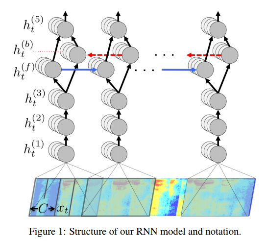
DS1 Architecture
RNN: 3 non-recurrent and 1 bi-directional recurrent layer, 1 non-recurrent
- Input: spectrogram
- Output: sequence of character probabilities
- Decoding: 5-gram language model
- Loss function: CTC
- Nesterov's Accelerated Gradient Descent (evolution of gradient descent)
Decoding with Language Model
Reduce WER by including language model:
$\underset{y}{\operatorname{argmax}}Q(y) = log(p_ctc(y \mid x)) + \alpha * log(p_lm(y)) + \beta * word\_count(y)$
- $\alpha$: relative weight of language model vs. CTC
- $\beta$: considers more words
Beam search: take $k$ best $y$ on every iteration, similar to breath-first-search but with beam width $k$

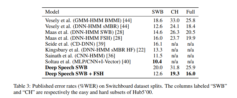
(image: DeepSpeech paper)
Dataset Construction
- Synthesize noisy speech by overlaying tracks
- Lombard Effect: play loud background noise while recording so that speaker will raise their pitch
DeepSpeech 2
- Same model recognizes multiple languages (English or Mandarin Chinese)
- no separate pronounciation model needed
- Parellel GPU training optimizations cut down training & iteration times
- GPU implementation of CTC
- custom memory allocators
DS2 Architecture
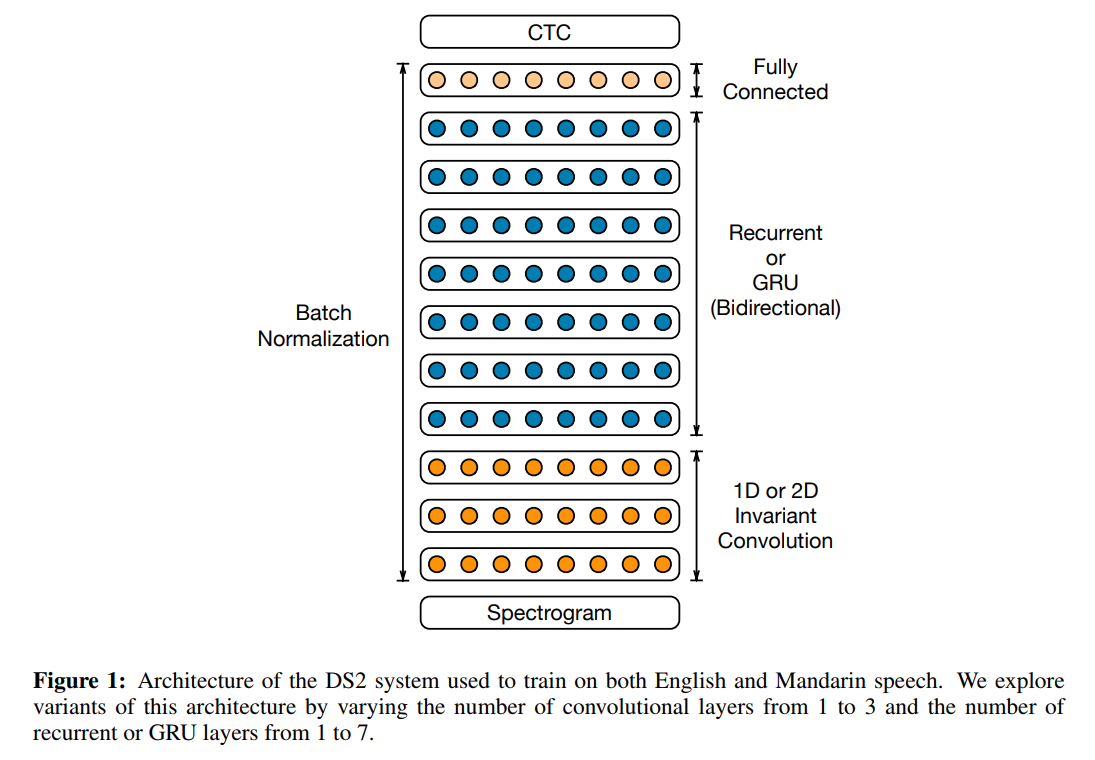
- More layers (recurrent, convolutional)
- Batch Normalization
- SortaGrad learning strategy
(image: DeepSpeech 2 paper)
Batch Normalization
- Original paper: https://arxiv.org/abs/1502.03167
$$B(x) = \gamma \frac{x - Mean[x]}{(Variance[x] + \epsilon)^\frac{1}{2}} + \beta $$
- $Mean[x]$, $Variance[x]$: Minibatch mean and variance
- $\gamma$, $\beta$: learned parameters
- $\epsilon$: small constant to avoid division by zero
- Typically applied before activation $f(x)$: $$h^l = f(B(W^lh^{l-1}))$$
- For bidirectional RNNs, Batch Norm is applied sequence-wise: $$h^l_t = f(B(W^lh^{l-1}) + U^lh^l_{t-1})$$
Batch Normalization Effect
- Generally: speeds up convergence by removing "uninteresting" changes in mean and variance ("internal covariate shift")
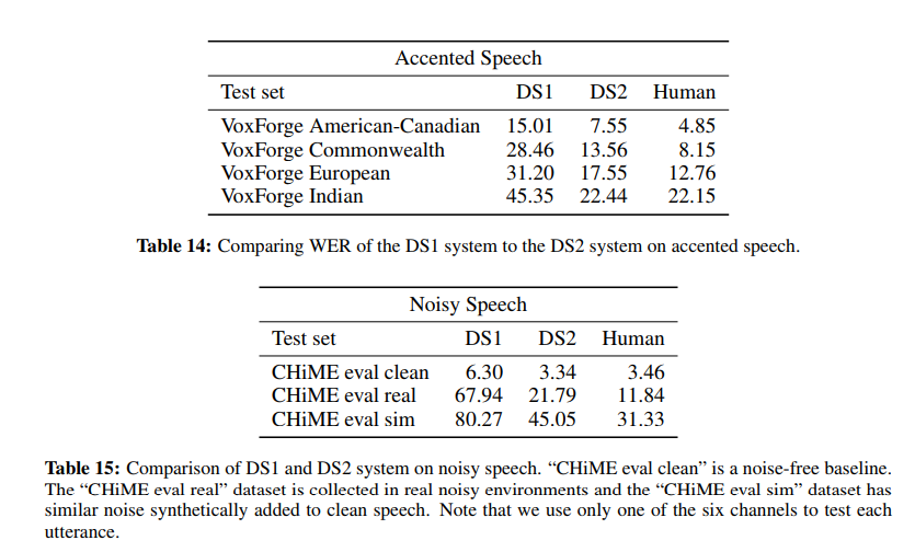
- Deep Speech 2: improved generalization error by as much as 12%
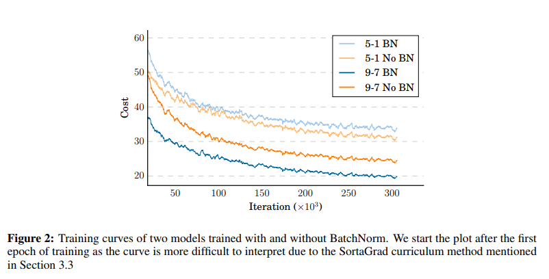
(image: DeepSpeech 2 paper)
SortaGrad (Curriculum Strategy)
- Longer utterances usually have higher CTC cost than shorter utterances
- Early in training: susceptible to numerical instabilities like underflow, exploding gradient
- Solution
- During the first epoch, sort utterances so that shorter utterances are encountered first
- Subsequent epochs: revert to random order

(image: DeepSpeech 2 paper)
Decoding
Fuse acoustic model with language model:
$$Q(y) = log(p_ctc(y \mid x)) + \alpha * log(p_lm(y)) + \beta * word\_count(y)$$
- $\alpha$: relative weight of language model vs. CTC
- $\beta$: considers more words
Language model
- n-gram: scales to large quantities of unlabeled text
- English: 850 million n-grams
- Mandarin: 2 billion n-grams (character level).
- Output layer is 6000 characters
- includes English alphabets to handle mixed Chinese-English transcripts
Dataset Construction
Pipeline
- Birectional RNN with CTC to align transcription to audio
- Segmentation: splice audio between long silences, average 7s length
- Linear classifier to predict bad examples from failed alignments, using crowd sourced ground truth transcriptions
Data augmentation by adding noise to 40% of random utterances
- too much noise makes optimization difficult
- too little noise makes system less robust to noisy speech
Deep Speech Workshop Setup
Repo: https://github.com/mozilla/DeepSpeech
DeepSpeech requires Ubuntu, run the following commands from an Ubuntu machine.
conda create --name deepspeech
source activate deepspeech
pip3 install jupyter matplotlib python_speech_features --user

# If running without GPU
pip3 install deepspeech

# If running on GPU
pip3 install deepspeech-gpu

# Download pre-trained models (approx. 1.4GB)
curl -o deepspeech-0.1.1-models.tar.gz -L https://github.com/mozilla/DeepSpeech/releases/download/v0.1.1/deepspeech-0.1.1-models.tar.gz

# Extract
tar -xvzf deepspeech-0.1.1-models.tar.gz

# Install SoX to convert audio to single channel 16kHz PCM
# needed by DeepSpeech
sudo apt-get install -y sox

# Launch Jupyter and browse to this notebook
jupyter notebook# Ref: https://github.com/mozilla/DeepSpeech/blob/master/native_client/python/client.py
from deepspeech.model import Model
import numpy as np
# Model
MODEL_GRAPH = 'models/output_graph.pb'
LANGUAGE_MODEL = 'models/lm.binary'
LM_ALPHABET = 'models/alphabet.txt'
LM_TRIE = 'trie'
Input Processing
We'll define a helper function prepare_input that prepares the input to match the training data characteristics:
- Sample rate of 16kHz
- Duration of 6 seconds
We'll also define another function visualize_input that plots the spectrogram of the audio sample.
def prepare_input(audio_path):
    """Ensures audio matches the sample rate supported by Deep Speech,
       and truncates the audio to the required length.
    Args:
        audio_path: path ot the audio file
    Returns:
        A tuple with (sample_rate, converted_audio)
    """
    import subprocess
    import scipy.io.wavfile as wav
    sample_rate = 16000
    duration_secs = 6

    fs, audio = wav.read(audio_path)
    if fs != sample_rate:
        if fs < sample_rate:
            print('Warning: original sample rate (%d) is lower than 16kHz. Up-sampling might produce erratic speech recognition.' % (fs), file=sys.stderr)

        print('Resampling audio from {}kHz to 16kHz'.format(fs/1000))
        sox_cmd = 'sox {} --type raw --bits 16 --channels 1 --rate {} - '.format(audio_path, sample_rate)
        try:
            p = subprocess.Popen(sox_cmd.split(),
                                 stderr=subprocess.PIPE, stdout=subprocess.PIPE)
            output, err = p.communicate()

            if p.returncode:
                raise RuntimeError('SoX returned non-zero status: {}'.format(err))

        except OSError as e:
            raise OSError('SoX not found, use 16kHz files or install it: ', e)

        audio = np.fromstring(output, dtype=np.int16)

    # Truncate to smaller length, as DeepSpeech is trained on
    # short utterances (a few seconds long)
    print('Truncating audio from {}s to {}s'.format(len(audio)/sample_rate, duration_secs))

    max_frames = sample_rate * duration_secs
    audio = audio[:max_frames]
    return sample_rate, audio

def visualize_input(sample_rate, audio, title):
    """Plots an audio spectrogram and shows a player for it
    Args:
        sample_rate: sample rate
        audio: audio sample buffer
        title: plot title
    """
    import matplotlib.pyplot as plt
    from python_speech_features import mfcc
    from scipy.io.wavfile import read

    # plot spectrogram
    features = mfcc(audio, sample_rate, winlen=0.025, winstep=0.01,
                    numcep=26, appendEnergy=False)

    fig, ax = plt.subplots(nrows=1, ncols=1, figsize=(20,4))
    cax = ax.matshow(np.transpose(features), interpolation='nearest',
                     aspect='auto', cmap='plasma', origin='lower')
    fig.colorbar(cax)

    plt.title(title)
    plt.show()
Test input
Just for fun, we'll try a corpus of Singapore English.
You can find examples from the NIE Corpus of Spoken Singapore English
For comparison, we'll generate a US English sample using an online text-to-speech generator
# Try something from the NIE Corpus of Spoken Singapore English
# http://videoweb.nie.edu.sg/phonetic/niecsse/index.htm
transcription = 'the north wind and the sun were disputing which was the stronger when a traveler came along'

# Singaporean English
!curl -o singaporean.wav -L 'http://videoweb.nie.edu.sg/phonetic/niecsse/nws/nws-SE-f1.WAV'

# ==================================================================
# American English
# 1. Go to https://www.text2speech.org in your browser
# 2. Generate a speech sample using the transcription text above
# 3. Replace the link to the .wav
!curl -o american.wav -L 'PASTE_YOUR_LINK_HERE'


sample_rate1, audio1 = prepare_input('singaporean.wav')
sample_rate2, audio2 = prepare_input('american.wav')

visualize_input(sample_rate1, audio1, "Singaporean English")
visualize_input(sample_rate2, audio2, "American English")
Perform the inference
- Load the acoustic model
- Enable language model decoding
# Constants
# These constants control the beam search decoder
# Beam width used in the CTC decoder when building candidate transcriptions
BEAM_WIDTH = 500

# The alpha hyperparameter of the CTC decoder. Language Model weight
LM_WEIGHT = 1.75

# The beta hyperparameter of the CTC decoder. Word insertion weight (penalty)
WORD_COUNT_WEIGHT = 1.00

# Valid word insertion weight. This is used to lessen the word insertion penalty
# when the inserted word is part of the vocabulary
VALID_WORD_COUNT_WEIGHT = 1.00

# These constants are tied to the shape of the graph used (changing them changes
# the geometry of the first layer), so make sure you use the same constants that
# were used during training

# Number of MFCC features to use
N_FEATURES = 26

# Size of the context window used for producing timesteps in the input vector
N_CONTEXT = 9

# Load the acoustic model
ds = Model(MODEL_GRAPH, N_FEATURES, N_CONTEXT, LM_ALPHABET, BEAM_WIDTH)
print('Loaded model')

# Load the language model
ds.enableDecoderWithLM(LM_ALPHABET, LANGUAGE_MODEL, LM_TRIE, LM_WEIGHT,
                       WORD_COUNT_WEIGHT, VALID_WORD_COUNT_WEIGHT)

print('Loaded language model')

# ==================================================================
# Exercise:
# Add code below to get the evaluation result for both audio samples
#
# Use ds.stt(), see an example at:
# https://github.com/mozilla/DeepSpeech/blob/master/native_client/python/client.py

result1 = '' # replace this with your code


result2 = '' # replace this with your code


print('Original:', transcription)
print('Singaporean:', result1)
print('American:', result2)
Evaluate metrics
We'll compute the edit distance of the two text transcriptions (the actual vs. predicted) to determine how far apart they are.
Refer to http://www.nltk.org/howto/metrics.html for the available metrics, and complete the code below.
def evaluate_metrics(truth, prediction):
    """Returns a metric indicating how good the prediction is
       This should be the word error rate.
    Args:
        prediction: the prediction
        truth: the correct value
    """
    # ==================================================================
    # Complete the code below, using nltk.metrics.edit_distance


    pass

print('Singaporean:', evaluate_metrics(transcription, result1))
print('American:', evaluate_metrics(transcription, result2))
Training Environment
- Documentation: https://github.com/mozilla/DeepSpeech#training
- Ubuntu + GPU is required for actual training.
- Even if you don't have a GPU machine readily available, you should try this using CPU.
Create environment
conda create --name deepspeech-train
source activate deepspeech-train
conda install pip
Clone
git clone https://github.com/mozilla/DeepSpeech.gitInstall requirements
cd DeepSpeech
pip install -r requirements.txt
python util/taskcluster.py --target .

# Install libdeepspeech.so, otherwise training scripts will emit warning about it
pip install deepspeech

## hack to get the provided training scripts to work
cd native_client
ln -s libctc_decoder_with_kenlm.so .
cd ..
If running on GPU: install TensorFlow GPU
pip uninstall tensorflow --user
pip install 'tensorflow-gpu==1.6.0' --user
Overfit Small Dataset
First, we'll validate our setup by overfitting a small dataset. We'll use the toy LDC93S1 dataset, which contains just 1 utterance.
Open bin/run-ldc93s1.sh in an editor and inspect it. It contains two parts:
- Downloading and importing the dataset
- Training using
Deepspeech.py
We'll use this script as a reference for setting up DeepSpeech training for other datasets.
Training
Start training from the DeepSpeech top level directory:
bin/run-ldc93s1.shEven without a GPU, this should take less than 10 minutes to complete.
I FINISHED Optimization - training time: 0:01:08
I Test of Epoch 50 - WER: 0.818182, loss: 12.298973083496094, mean edit distance: 0.173077
I --------------------------------------------------------------------------------
I WER: 0.818182, loss: 12.298973, mean edit distance: 0.173077
I  - src: "she had your dark suit in greasy wash water all year"
I  - res: "she had yorodarksuitingreasywashwaterallyear"
I --------------------------------------------------------------------------------
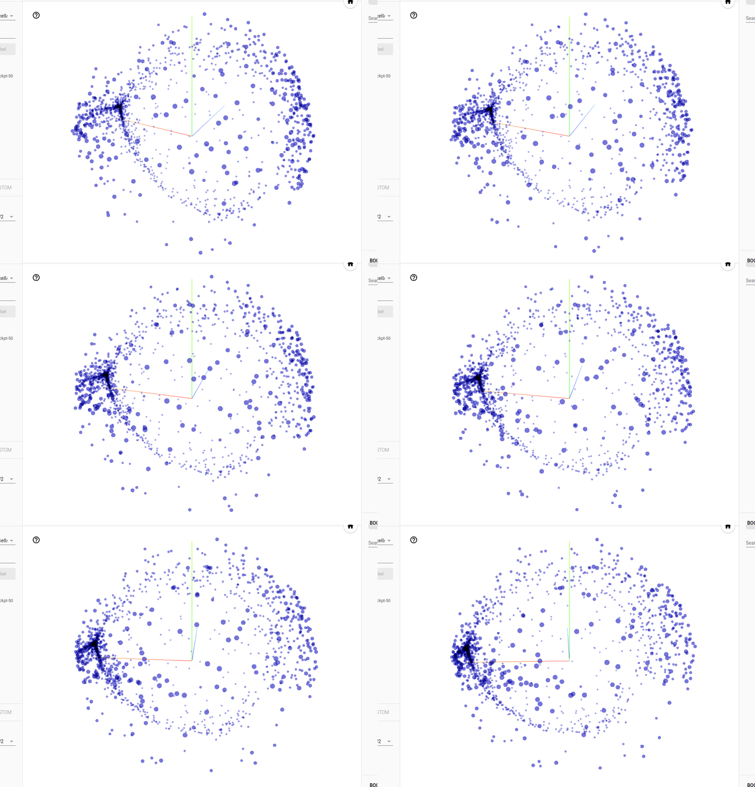
Training output and TensorBoard
By default, training only saves checkpoint files. The default location is $HOME/.local/share/deepspeech/ldc93s1.
This includes TensorBoard log files. To explore the TensorBoard graphs, you can run:
tensorboard --logdir $HOME/.local/share/deepspeech/ldc93s1Follow the prompts to open the browser to http://localhost:6006. Discover something cool like the PCA projection of the gate weights of an LSTM cell:
Exporting / freezing models
To fine tune a model or release the model for others to use, convert the checkpoint files to a model file. This is done by passing the --export_dir flag to the training script.
Run this from the DeepSpeech top level directory:
mkdir models
bin/run-ldc93s1.sh --export_dir models
When done, you should see output_graph.pb in the models directory. We will need it for the next section.
Checkpointing as a Best Practice
Note that the training script stores state in the checkpoint directory, so that it resumes from the previous checkpointed state upon reruns. This is critical for long running training sessions where the system may crash. Checkpoints allow the training to recover and resume.
Fine-tuning
Now that we've trained our toy model, let's practice fine tuning it. We'll try some new data from the NIE Singapore English Corpus.
Data Processing
The data needs to be processed to 16kHz and chopped into 6-7 second utterances.
The transcription also needs to be split and aligned with the data. This is done manually by listening to each chopped up wav file and finding the matching transcription.
Full text:
The North Wind and the Sun were disputing which was the stronger when a traveler came along wrapped in a warm cloak. They agreed that the one who first succeeded in making the traveller take his cloak off should be considered stronger than the other. Then the North Wind blew as hard as he could, but the more he blew the more closely did the traveller fold his cloak around him; and at last the North Wind gave up the attempt. Then the Sun shone out warmly, and immediately the traveller took off his cloak. And so the North Wind was obliged to confess that the Sun was the stronger of the two.In practice, getting the transcription truth is one of the more time-consuming parts of data gathering. This is usually done by humans through crowdsourcing efforts like the Common Voice Corpus.
import IPython

IPython.display.Audio("http://videoweb.nie.edu.sg/phonetic/niecsse/nws/nws-SE-f1.WAV")
Running the import script
Save the script below in the DeepSpeech top level directory and run it.
import_nie.pyWhen done, your data set should look like:
data/nws-SE-f1-test.csv      data/nws-SE-f1-train.csv
data/nws-SE-f1_chunk001.wav  data/nws-SE-f1_chunk004.wav
data/nws-SE-f1_chunk002.wav  data/nws-SE-f1_chunk005.wav
data/nws-SE-f1_chunk003.wav  data/nws-SE-f1_chunk006.wav
data/nws-SE-f1_chunk007.wav
Note chunk007 will not be used for training or testing (it contains only silence)
#!/usr/bin/env python
"""Importer script to create a sample NIE Singapore English Speech DeepSpeech dataset

Save this script to the DeepSpeech directory and run it without any arguments:
   import_nie.py
"""

import os
import pandas
import subprocess

def _resample_and_split_audio(audio_path, sample_rate=16000, chunksize_secs=6):
    """Resamples and splits the input audio into chunks.
    Args:
        audio_path: path to the input audio.
        sample_rate: target sample rate (Hz).
        chunksize_secs: target chunk size (seconds).
    Returns:
        Array of paths to the split audio.
    """
    import glob
    import scipy.io.wavfile as wav
    audio_path_noext = os.path.splitext(audio_path)[0]

    fs, _ = wav.read(audio_path)
    if fs != sample_rate:
        if fs < sample_rate:
            print('Warning: original sample rate ({}) is lower than {}Hz. \
                Up-sampling might produce erratic speech recognition.'.\
                format(fs, sample_rate), file=sys.stderr)

    print('Resampling audio to {}Hz'.format(sample_rate))

    # SoX reference: http://sox.sourceforge.net/sox.html
    # sox foo.wav --rate 16000 --bits 16 --channels 1 foo_resampled.wav
    sox_cmd = 'sox {} --rate {} --bits 16 --channels 1 {}_resampled.wav'.\
        format(audio_path, sample_rate, audio_path_noext)
    try:
        p = subprocess.Popen(sox_cmd.split(),
                             stderr=subprocess.PIPE, stdout=subprocess.PIPE)
        _, err = p.communicate()

        if p.returncode:
            raise RuntimeError('SoX returned non-zero status: {}'.format(err))

        print('Splitting audio into {}s chunks'.format(chunksize_secs))

        # sox foo_resampled.wav foo_chunk.wav trim 0 6 : newfile : restart
        sox_cmd = 'sox {}_resampled.wav {}_chunk.wav trim 0 {} : newfile : restart'.\
            format(audio_path_noext, audio_path_noext, chunksize_secs)
        p = subprocess.Popen(sox_cmd.split(),
                             stderr=subprocess.PIPE, stdout=subprocess.PIPE)
        _, err = p.communicate()

        if p.returncode:
            raise RuntimeError('SoX returned non-zero status: {}'.format(err))
    except OSError as e:
        raise OSError('SoX not found, use {}Hz files or install it: '.format(sample_rate), e)

    # list of chunked files
    return sorted(glob.glob('{}_chunk*.wav'.format(audio_path_noext)))

def maybe_download(filename, work_directory, source_url):
  """Download the data from source url, unless it's already here.
  Args:
      filename: string, name of the file in the directory.
      work_directory: string, path to working directory.
      source_url: url to download from if file doesn't exist.
  Returns:
      Path to resulting file.
  """
  import shutil
  import urllib

  if not os.path.exists(work_directory):
      os.makedirs(work_directory)
  filepath = os.path.join(work_directory, filename)

  if not os.path.exists(filepath):
    temp_file_name, _ = urllib.request.urlretrieve(source_url, filename)
    shutil.move(temp_file_name, filepath)
    print('Successfully downloaded', filename, os.path.getsize(filepath), 'bytes.')
  return filepath

def _download_and_preprocess_data(data_dir):
    import re
    NWS_SE_F1_WAV = "nws-SE-f1.wav"
    NWS_SE_F1_WAV_URL = "http://videoweb.nie.edu.sg/phonetic/niecsse/nws/nws-SE-f1.WAV"

    # transcript that's pre-chunked into 6 second speech.
    # this is done by manually playing back each chunk.
    NWS_SE_F1_TXT = [
        "The North Wind and the Sun were disputing which was the stronger when a traveler came along",
        "wrapped in a warm cloak. They agreed that the one who first succeeded in making the traveller take his cloak",
        "off should be considered stronger than the other. Then the North Wind blew as hard as he could, but the",
        "more he blew the more closely did the traveller fold his cloak around him; and at last the North Wind gave up the",
        "attempt. Then the Sun shone out warmly, and immediately the traveller",
        "took off his cloak. And so the North Wind was obliged to confess that the Sun was the stronger of the two.",
        " "] # silence

    local_file = maybe_download(NWS_SE_F1_WAV, data_dir, NWS_SE_F1_WAV_URL)

    # lowercase, remove extra spacing
    transcripts = [text.strip().lower() for text in NWS_SE_F1_TXT]

    # remove anything other than characters and space
    transcripts = [re.sub(r'[^\w\s]', '', text) for text in transcripts]

    # process the audio files
    audio_files = _resample_and_split_audio(local_file)

    # sanity check
    if len(audio_files) != len(transcripts):
        raise RuntimeError('number of chunked files ({}) != number of transcripts ({})'. \
            format(len(audio_files) , len(transcripts)))

    # drop silence (last transcript)
    audio_files = [audio_files[i] for i in range(0, len(transcripts)) if len(transcripts[i]) > 0]

    # create the data frame, reserving last 2 entries as test data
    data = [(os.path.abspath(audio_files[i]), os.path.getsize(audio_files[i]), transcripts[i])
        for i in range(0, len(audio_files))]

    df = pandas.DataFrame(data=data[:len(data)-2],
                          columns=["wav_filename", "wav_filesize", "transcript"])
    df.to_csv(os.path.join(data_dir, "nws-SE-f1-train.csv"), index=False)
    print("Created:", os.path.join(data_dir, "nws-SE-f1-train.csv"))

    df = pandas.DataFrame(data=data[len(data)-2:],
                          columns=["wav_filename", "wav_filesize", "transcript"])
    df.to_csv(os.path.join(data_dir, "nws-SE-f1-test.csv"), index=False)
    print("Created:", os.path.join(data_dir, "nws-SE-f1-test.csv"))

if __name__ == "__main__":
    _download_and_preprocess_data(data_dir='data')
Fine-tuning from a frozen model
Ref: https://github.com/mozilla/DeepSpeech#continuing-training-from-a-frozen-graph
Run these commands that will:
- Initialize from the model that we saved earlier
- Save the checkpoints to a new checkpoint location for this fine-tuning session
- Run the fine-tuning session for 50 epochs with a small learning rate
mkdir fine_tuning_checkpoints

python -u DeepSpeech.py \
  --n_hidden 494 \
  --initialize_from_frozen_model models/output_graph.pb \
  --checkpoint_dir fine_tuning_checkpoints \
  --train_files data/nws-SE-f1-train.csv \
  --dev_files data/nws-SE-f1-train.csv \
  --test_files data/nws-SE-f1-test.csv \
  --learning_rate 0.0001
  --epoch 50 \
You should see output that looks like:
(deepspeech-train) $ python -u DeepSpeech.py \
>   --n_hidden 494 \
>   --initialize_from_frozen_model models/output_graph.pb \
>   --checkpoint_dir fine_tuning_checkpoints \
>   --train_files data/nws-SE-f1-train.csv \
>   --dev_files data/nws-SE-f1-train.csv \
>   --test_files data/nws-SE-f1-test.csv \
>   --learning_rate 0.0001
W Parameter --validation_step needs to be >0 for early stopping to work
I Initializing from frozen model: models/output_graph.pb
I STARTING Optimization
I Training of Epoch 0 - loss: 748.212051
I Training of Epoch 1 - loss: 630.433716
I Training of Epoch 2 - loss: 566.069580
I Training of Epoch 3 - loss: 512.083084
I Training of Epoch 4 - loss: 472.369240
I Training of Epoch 5 - loss: 433.883522
I Training of Epoch 6 - loss: 403.633568
I Training of Epoch 7 - loss: 373.490967
I Training of Epoch 8 - loss: 346.342918
Practice Exercises
- Try fine-tuning with different hyper-parameters, such as learning rate. Note that the number of hidden layers is fixed by the frozen model
- Try training an initial model with a Singapore English sample instead, then fine-tuning it with more Singapore English samples
- Investigate creating a language model for Singapore English to improve the transcription result
