Topics
- Linear and polynomial equations
- Loss functions
- Gradient descent
- Evaluation metrics
- Appendix: Regularized Regression Models
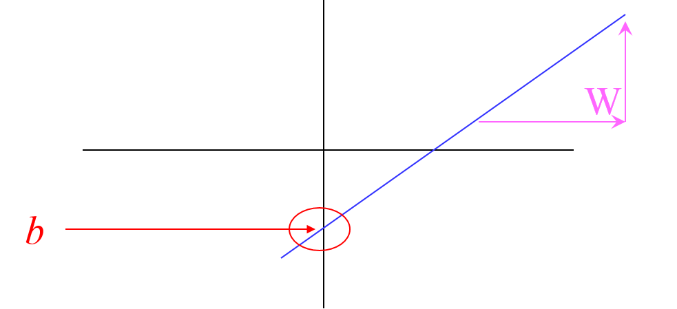
Linear Equation
From $x$ (a feature), predict $y$ (outcome or result) assuming a "linear relationship".
$$y=Wx+b$$
Objective
Given $y = Wx+b$
Find $W$ and $b$ so that $y$ is as accurate as possible
Loss function: measures "how accurate"
Loss Functions
Also known as cost function, objective function
Example: Mean Square Error $$L(W, b) = MSE(W, b) = \frac{1}{N}\sum_{i=1}^N{\big(y_i - (Wx_i + b)\big)^2}$$
Many more examples: http://scikit-learn.org/stable/modules/model_evaluation.html
Objective (of Training)
Find $W^*$ and $b^*$ to minimize the loss function:
$$\underset{W^*, b^*}{\arg \min}\; L(W, b)$$
$$\underset{W^*, b^*}{\arg \min}\; \frac{1}{N}\sum_{i=1}^N{\big(y_i - (Wx_i + b)\big)^2}$$
$N$: number of samples
Gradient Descent
- Initialize parameters ($W$ and $b$) to random values
- Compute gradient of the loss function: $L'(W, b)$
- Update rule ($\epsilon$ = learning rate) $$W := W -\epsilon L'(W, b)$$ $$b := b -\epsilon L'(W, b)$$
- Repeat 2 and 3 until find $W^*$ and $b^*$
Linear Equation as Dot Product
$y = Wx + bx_0 = bx_0 + Wx$
$y = \left[ \begin{array}{cc} b & W \end{array} \right] \left[ \begin{array}{c} x_0 \\ x \end{array} \right] = \left[ \begin{array}{cc} b & W \end{array} \right] \left[ \begin{array}{c} 1 \\ x \end{array} \right] = \left[ \begin{array}{c} b \\ W \end{array} \right]^T \left[ \begin{array}{c} 1 \\ x \end{array} \right] = \theta^TX$
where $\theta = \left[ \begin{array}{c} b \\ W \end{array} \right]$ and $X = \left[ \begin{array}{c} 1 \\ x \end{array} \right]$
Polynomial Equation as Dot Product
$y = W_2x^2 + W_1x + b = b+ W_1x + W_2x^2$
$y = \left[ \begin{array}{ccc} b & W_1 & W_2 \end{array} \right] \left[ \begin{array}{c} 1 \\ x \\ x^2 \end{array} \right] = \left[ \begin{array}{c} b \\ W_1 \\ W_2 \end{array} \right]^T \left[ \begin{array}{c} 1 \\ x \\ x^2\end{array} \right] = \theta^TX$
Loss Function
For the $i^{th}$ sample: $y_i = \theta^TX_i$
Loss function computes for all N samples: $$L(\theta) = MSE(\theta) = \frac{1}{N}\sum_{i=1}^N{\big(y_i - \theta^TX_i\big)^2}$$
Why Dot Product?
import numpy as np

# 25 features, 10000 samples
X = np.random.rand(10000, 25)
W = np.random.rand(1, 25)

y1 = np.zeros((10000, 1))
%%time
for i in range(X.shape[0]):
    for j in range(X.shape[1]):
     y1[i] = y1[i] +W[0][j]*X[i][j]
%time
y2 = np.dot(X, W.T)
# ensure the two operations are the same
np.testing.assert_allclose(y1, y2)
Libraries
http://scikit-learn.org/stable/modules/linear_model.html#linear-model
- LinearRegression (Least Squares)
- PolynomialFeatures
Evaluation Metrics
http://scikit-learn.org/stable/modules/model_evaluation.html#regression-metrics
- Mean squared error (MSE): standard measure, but meaningless for exponentially large values
- Mean squared log error (MSLE): use for exponentially large values
- Mean absolute error (MAE): less sensitive to large errors than MSE / MSLE (which squares them)
- $R^2$ score: Generally convenient to use for scoring, because higher number is better, and range is usually 0 to 1.
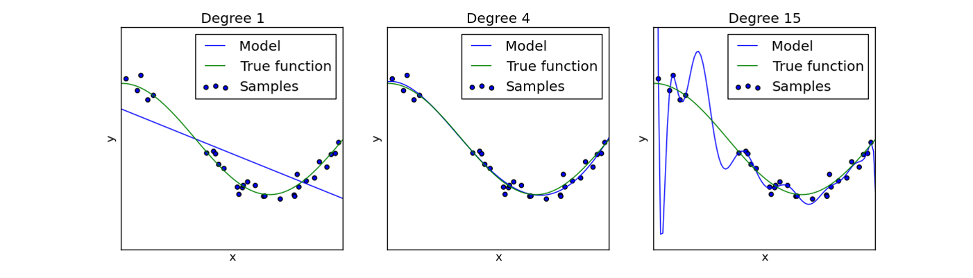
Appendix: Regularized Regression Models
Here's a quick summary of other regression models that may be of interest.
- Ridge Regression: applies L2 regularization
- Lasso: applies L1 regularization
- Elastic Net: applies L1 and L2 regularization
L1 vs. L2 Regularization
| L1 Regularization | L2 Regularization |
|---|---|
| Uses sum of squares of weights | Uses sum of weights |
| Computationally efficient, differentiable | Less computationally efficient, not differentiable |
| Produces sparse outputs because sum can cancel out weights | Produces non-sparse outputs |
Recap: Linear Regression
Objective:
$$\underset{w} {\arg \min} {\left\Vert Xw - y \right\Vert_2}^2 $$
When there are multiple features in $X$, assumes features are independent.
If not, least squares becomes sensitive to noise. This is because the same noise can appear in related features and be magnified.
Note:
This syntax ${\left\Vert Xw - y \right\Vert_2}^2$ means the residual sum of squares: $\sum_i^n {(X_iw - y_i)}^2$
%matplotlib notebook
import matplotlib.pyplot as plt
import numpy as np
from mpl_toolkits.mplot3d import Axes3D

# Our fake data
X = [[0, 0], [0, 0], [1, 1]]
y = [0, .1, 1]

# Let's plot our fake data in 3D
# We need 3 columns: x0, x1, y
data = np.array(X)
X0 = data[:, 0]
X1 = data[:, 1]

fig, ax = plt.subplots(subplot_kw=dict(projection='3d'))
ax.scatter(X0, X1, y)
ax.set(xlabel='X0', ylabel='X1', zlabel='y')
fig.show()
from sklearn.linear_model import LinearRegression

# Our baseline model
model = LinearRegression()

model.fit(X, y)
print('Coefficients', model.coef_, 'Intercept', model.intercept_)

X_test = [[1, 1]] # needs to be 2D array
model.predict(X_test)
def plot_model(model, X, ax, label, color):
    """Plots a model on the given axes
    Args:
        model: the model to plot
        X: the input data
        ax: the matplotlib axes
        label: the label for the plot
        color: the color of the plot
    """
    data = np.array(X)
    X0 = data[:, 0]
    X1 = data[:, 1]

    x_test = np.stack((np.linspace(min(X0), max(X0)),
                   np.linspace(min(X1), max(X1))),
                  axis=1)
    preds = model.predict(x_test)
    ax.plot(x_test[:, 0], x_test[:, 1], preds, label=label, color=color)
# Plot the model against samples
fig, ax = plt.subplots(subplot_kw=dict(projection='3d'))

# plot the samples
ax.scatter(X0, X1, y, label='data')

# plot the model
plot_model(model, X, ax, 'linear regression', 'red')

ax.set(xlabel='X0', ylabel='X1', zlabel='y')
ax.legend()
fig.show()
Ridge Regression
Linear Regression + L2 Regularization = Ridge Regression
Penalizes the input features by a factor of the sum-of-squares of the parameters.
Objective:
$$\underset{w} {\arg \min} {\left\Vert Xw - y \right\Vert_2}^2 + \alpha {\left\Vert w \right\Vert_2}^2 $$
$\alpha$ = regularization hyperparameter. Increase this when you suspect input features have higher linear dependencies.
Notes:
- This syntax ${\left\Vert w \right\Vert_2}^2$ means $\sum_1^k {w_j}^2$, where $k$ is the number of parameters
# http://scikit-learn.org/stable/modules/linear_model.html#ridge-regression
from sklearn.linear_model import Ridge

alpha = .5
ridge = Ridge(alpha=alpha)

ridge.fit(X, y)
print('Coefficients', ridge.coef_, 'Intercept', ridge.intercept_)

X_test = [[1, 1]] # needs to be 2D array
ridge.predict(X_test)
# Plot the models against samples
fig, ax = plt.subplots(subplot_kw=dict(projection='3d'))

# plot the samples
ax.scatter(X0, X1, y, label='data')

# plot the models
plot_model(model, X, ax, 'linear regression', 'red')
plot_model(ridge, X, ax, 'ridge (alpha %.2f)' % alpha, 'green')

ax.set(xlabel='X0', ylabel='X1', zlabel='y')
ax.legend()
fig.show()
# Same as above, but using cross-validated search
# on a selection of alpha values (like GridSearchCV)
from sklearn.linear_model import RidgeCV

alphas = [1e3, 1e2, 0.1, 1.0, 10]

ridge_cv = RidgeCV(alphas=alphas)
ridge_cv.fit(X, y)

print('Coefficients', ridge_cv.coef_, 'Intercept', ridge_cv.intercept_, 'Best alpha', ridge_cv.alpha_)

X_test = [[1, 1]] # needs to be 2D array
ridge_cv.predict(X_test)
# Plot the models against samples
fig, ax = plt.subplots(subplot_kw=dict(projection='3d'))

# plot the samples
ax.scatter(X0, X1, y, label='data')

# plot the models
plot_model(model, X, ax, 'linear regression', 'red')
plot_model(ridge, X, ax, 'ridge (alpha %.2f)' % alpha, 'green')
plot_model(ridge_cv, X, ax, 'ridge CV (alpha %.2f)' % ridge_cv.alpha_, 'black')

ax.set(xlabel='X0', ylabel='X1', zlabel='y')
ax.legend()
fig.show()
Ridge CV came up with a model that has better fit (closer to baseline).
Alpha of 0.5 is probably too much penalty on X0 and X1.
Lasso Regression
Linear Regression + L1 Regularization = Lasso
Penalizes the input features by a factor of the sum of the parameters.
- Tends to result in fewer coefficients (i.e. sparser model)
- More inefficient to compute
Objective:
$$\underset{w} {\arg \min} \frac{1}{2n} {\left\Vert Xw - y \right\Vert_2}^2 + \alpha {\left\Vert w \right\Vert_1} $$
$\alpha$ = regularization hyperparameter. Increase this when you suspect input features have higher linear dependencies.
Notes:
- This syntax ${\left\Vert w \right\Vert_1}$ means $\sum_1^k {w_j}$, where $k$ is the number of parameters
# http://scikit-learn.org/stable/modules/linear_model.html#lasso
from sklearn.linear_model import Lasso

alpha = .5
lasso = Lasso(alpha=alpha)

lasso.fit(X, y)
print('Coefficients', lasso.coef_, 'Intercept', lasso.intercept_)

X_test = [[1, 1]] # needs to be 2D array
lasso.predict(X_test)
# Plot the models against samples
fig, ax = plt.subplots(subplot_kw=dict(projection='3d'))

# plot the samples
ax.scatter(X0, X1, y, label='data')

# plot the models
plot_model(model, X, ax, 'linear regression', 'red')
plot_model(ridge, X, ax, 'ridge (alpha %.2f)' % alpha, 'green')
plot_model(ridge_cv, X, ax, 'ridge CV (alpha %.2f)' % ridge_cv.alpha_, 'black')
plot_model(lasso, X, ax, 'lasso (alpha %.2f)' % alpha, 'orange')

ax.set(xlabel='X0', ylabel='X1', zlabel='y')
ax.legend()
fig.show()
# Same as above, but using cross-validated search
# on a selection of alpha values (like GridSearchCV)
from sklearn.linear_model import LassoCV

lasso_cv = LassoCV(alphas=alphas)
lasso_cv.fit(X, y)

print('Coefficients', lasso_cv.coef_, 'Intercept', lasso_cv.intercept_, 'Best alpha', lasso_cv.alpha_)

X_test = [[1, 1]] # needs to be 2D array
lasso_cv.predict(X_test)
# Plot the models against samples
fig, ax = plt.subplots(subplot_kw=dict(projection='3d'))

# plot the samples
ax.scatter(X0, X1, y, label='data')

# plot the models
plot_model(model, X, ax, 'linear regression', 'red')
plot_model(ridge, X, ax, 'ridge (alpha %.2f)' % alpha, 'green')
plot_model(ridge_cv, X, ax, 'ridge CV (alpha %.2f)' % ridge_cv.alpha_, 'black')
plot_model(lasso, X, ax, 'lasso (alpha %.2f)' % alpha, 'orange')
plot_model(lasso_cv, X, ax, 'lasso CV (alpha %.2f)' % lasso_cv.alpha_, 'purple')

ax.set(xlabel='X0', ylabel='X1', zlabel='y')
ax.legend()
fig.show()
Elastic Net
Linear Regression + L1 Reg + L2 Reg = ElasticNet
Tries to reap the benefits from both Ridge and Lasso (stability plus sparser model).
Objective:
$$\underset{w} {\arg \min} \frac{1}{2n} {\left\Vert Xw - y \right\Vert_2}^2 + \alpha\beta {\left\Vert w \right\Vert_1} + \frac{\alpha(1-\beta)}{2} {\left\Vert w \right\Vert_2}^2 $$
$\alpha$, $\beta$ = regularization hyperparameters
Optional Exercise: Elastic Net
Try comparing ElasticNet and ElasticNetCV in a similar way as the above examples.
Note that there are two hyperparameters to tune.