Coping with Dimensionality
Topics
- The Curse of Dimensionality
- Principal Component Analysis
- Singular Value Decomposition
- Linear Discriminant Analysis
Visualizing data
Humans can't visualize data in more than 3-D
The Curse of Dimensionality
As number of dimensions increase, need exponentially more data to create a generalized model
$d$ dimensions, $v$ target values: $O(v^d)$ examples
Dimension Reduction - Objective
"Project" data from high dimensions to lower dimensions
There will be data loss, but should be within acceptable limits
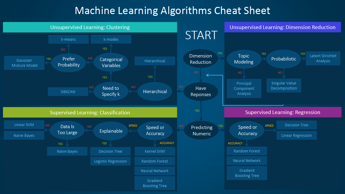
Dimension Reduction - Algorithms
- Principal Component Analysis (PCA)
- Singular Value Decomposition (SVD)
- Linear Discriminant Analysis
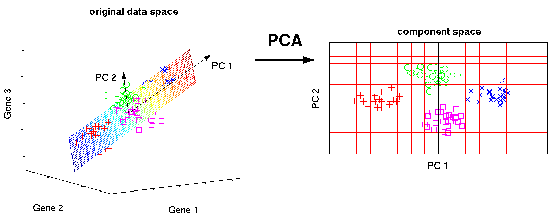
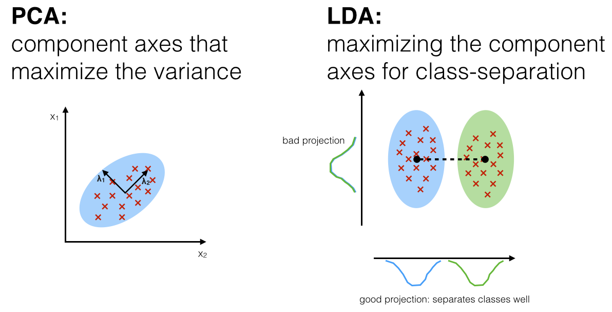
Principal Component Analysis
- 'Black box' matrix factorization / decomposition.
- Finds the subspace (defined by principal component axes) that can capture the highest variance
- Capturing the most variance minimizes information loss
- PCA is designed to be reversible (but not 100%)
PCA - Concept
To project $X$ from $p\,x\,n$ dimensions to $L\,x\,n$ dimensions: $$T_{L} = XW_{L}$$
- $X$: original matrix, $p\,x\,n$
- $W_{L}$: basis vector matrix $p\,x\,n$
- $T_{L}$: resulting projection of X, $L\,x\,n$
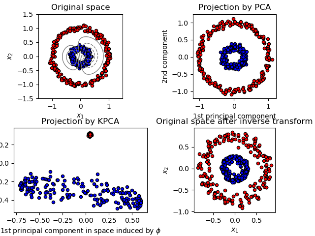
PCA - Types
http://scikit-learn.org/stable/modules/generated/sklearn.decomposition.PCA.html
- Linear PCA
- Kernel (non-linear) PCA
- linear, polynomial, radial basis function, sigmoid kernel functions
- Sparce PCA
- removes noise in the components due to matrix factorization
PCA - Steps
- Put with data into an $p\,x\,n$ matrix, where $p$ is number of features, $n$ is number of samples
- Zero-center by subtracting the mean
- Perform Singular vector (SVD) or Eigenvector Decomposition
PCA - Memory Constraints
- All data must fit in memory
- Larger datasets: use Incremental PCA: http://scikit-learn.org/stable/modules/decomposition.html#incremental-pca
Singular Value Decomposition
- An implementation of PCA
- A type of matrix factorization that uses singular matrices
SVD
$$T = XW = U\Sigma W^TW = U\Sigma$$
- $U$: left singular vectors of $X$, $n\,x\,n$
- $\Sigma$: singular matrix of $X$, $n\,x\,p$
- $W$: right singular vectors of $X$, $p\,x\,p$
Get $T_L = U_L \Sigma_L$ by truncating the first $L$ columns
Detailed explanation of PCA and SVD
A Tutorial on Principal Component Analysis: https://arxiv.org/abs/1404.1100
Linear Discriminant Analysis
- Supervised
- Uses the class labels to compute class separation of data
- Given $C$ classes, $p$ features, LDA can reduce features from $p$ into $C-1$ features.
- Dual purpose:
- Dimensionality reduction
- Classifier
Workshop - Data Projections
In this workshop, we will
- Perform 2-dimensional and 3-dimensional PCA projections, using SVD solvers, on a multi-dimensional dataset
- Perform Linear Discriminant Analysis to project that same dataset into n_classes - 1
Dataset - Motion Capture Hand Postures
5 types of hand postures from 12 users were recorded using unlabeled markers on fingers of a glove in a motion capture environment. Due to resolution and occlusion, missing values are common.
https://archive.ics.uci.edu/ml/datasets/Motion+Capture+Hand+Postures
- Download the data set from the link above
- Extract into a folder and update
read_csvto use your path
import pandas as pd

df = pd.read_csv('D:/tmp/Postures/Postures.csv') # update this to your path
df = df.apply(pd.to_numeric, errors='coerce') # convert non-numeric values to NaN
df.head(10)
# skip the first row, which is all zeros
df = df.iloc[1:]

# randomly sample 5000 points to plot
df = df.sample(n=5000)
print('df.shape:', df.shape)

# split into X and y (ignore User column)
X = df.loc[:, 'X0':]
y = df.loc[:, 'Class']

print('X.shape:', X.shape)
print('y.shape:', y.shape)
from sklearn.decomposition import PCA

# Run PCA to project into 2 components
pca = PCA(n_components=2)
X_pca = pca.fit_transform(X) # will fail
Exercise - Removing NaNs for PCA
If you try to run PCA directly above, you should see this error:
Input contains NaN, infinity or a value too large for dtype('float64').
In this exercise:
- Replace the NaN values using
sklearn.preprocessing.Imputer: http://scikit-learn.org/stable/modules/generated/sklearn.preprocessing.Imputer.html - Re-run PCA
- Plot the PCA projection
For step 1, try different imputation strategies ('mean', 'median', 'most_frequent') to see if they make a difference in the plot and PCA.explained_variance_ratio_
Note: sklearn.impute.SimpleImputer will replace sklearn.preprocessing.Imputer in future versions of sklearn.
# impute missing values because PCA can't handle it
# can't just dropna() because some classes will have no coverage
#
# http://scikit-learn.org/dev/auto_examples/plot_missing_values.html

from sklearn.preprocessing import Imputer

# Your code here


# Re-run PCA after fixing the data
pca = PCA(n_components=2)
X_pca = pca.fit_transform(X)

print('Before: X.shape', X.shape)
print('After: X.shape', X_pca.shape)

# Percentage of variance explained by the 2 components (higher is better)
print('PCA: explained variance ratio (first two components): %s'
      % str(pca.explained_variance_ratio_))
Plot the PCA projection in 2D.
import matplotlib.pyplot as plt
import numpy as np

# target names from the data webpage
target_names = ['fist', 'stop', 'point 1 finger', 'point 2 fingers', 'grab']
n_classes = len(target_names)

fig, ax = plt.subplots(figsize=(10, 10))

# https://matplotlib.org/examples/color/colormaps_reference.html
colors = [plt.cm.viridis(each)
          for each in np.linspace(0, 1, n_classes)]

for color, i, target_name in zip(colors, y.unique(), target_names):
    ax.scatter(X_pca[y == i, 0], X_pca[y == i, 1], color=color, alpha=.8,
               lw=.5, s=10, label=target_name)
ax.legend(loc='upper right', shadow=False, scatterpoints=1, fontsize='large')
ax.set(title='2-D PCA of MoCap Hand Postures dataset')
ax.axis('tight')
Walkthrough: PCA projection into 3D-space
We can also project the Hand Postures data into 3 components and do a 3-D plot.
Credits: http://scikit-learn.org/dev/auto_examples/decomposition/plot_pca_iris.html
pca_3d = PCA(n_components=3)
X_pca_3d = pca_3d.fit_transform(X)

print('Before: X.shape', X.shape)
print('After: X.shape', X_pca_3d.shape)

# Percentage of variance explained by the 3 components (higher is better)
print('PCA: explained variance ratio (first three components): %s'
      % str(pca_3d.explained_variance_ratio_))
Plot the PCA projection in 3D.
# make the plot interactive, since we're in 3D!
%matplotlib notebook

from mpl_toolkits.mplot3d import Axes3D

fig, ax = plt.subplots(subplot_kw=dict(projection='3d'), figsize=(10, 10))

colors = [plt.cm.viridis(each)
          for each in np.linspace(0, 1, n_classes)]

for color, i, target_name in zip(colors, y.unique(), target_names):
    ax.scatter(X_pca_3d[y == i, 0], X_pca_3d[y == i, 1], X_pca_3d[y == i, 2],
               s=10, color=color, label=target_name)

ax.legend(loc='upper right', shadow=False, scatterpoints=1, fontsize='large')
ax.set(title='3-D PCA of MoCap Hand Postures dataset')
ax.axis('tight')
Exercise: Linear Discriminant Analysis
We'll now try LDA.
LDA can project the dataset from 35 features to 4 features (n_classes - 1)
Tasks:
- Fit
sklearn.discriminant_analysis.LinearDiscriminantAnalysison X and y, with the default number of components - Plot the first 3 features in 3-D
# 1. Fit sklearn.discriminant_analysis.LinearDiscriminantAnalysis
# Your code here

from sklearn.discriminant_analysis import LinearDiscriminantAnalysis
# 2. Plot the first 3 components in 3-D
# Your code here
Workshop - Impact of Dimensionality
In this workshop, we will explore whether dimensionality reduction can improve a classification model.
We will:
- Train a Random Forest Clasifier using all 11 features
- Train Random Forest Classifiers with the projections of features into these dimensions:
- 2-dimensions
- 5-dimensions
- Compare the performances of all the above models
Dataset - Wine Quality
Two datasets are included, related to red and white vinho verde wine samples, from the north of Portugal. The goal is to model wine quality based on physicochemical tests (see [Cortez et al., 2009], Web Link).
https://archive.ics.uci.edu/ml/datasets/Wine+Quality
- Download the two .csv files from the link above into a folder of your choice
- Update
read_csvto use your folder path
import pandas as pd

# we'll use the smaller dataset
df = pd.read_csv('D:/tmp/wine-quality/winequality-red.csv', delimiter=';') # update this to your path
df = df.apply(pd.to_numeric, errors='coerce') # convert non-numeric values to NaN
df.head(10)
X = df.loc[:, 'fixed acidity':'alcohol']
y = df.loc[:, 'quality']
print('X.shape:', X.shape)
print('y.shape:', y.shape)
from sklearn.model_selection import train_test_split

train_X, test_X, train_y, test_y = train_test_split(X, y, test_size=.4)
Classification model with all 11 dimensions
from sklearn.ensemble import RandomForestClassifier
from sklearn.model_selection import GridSearchCV
from sklearn.metrics import classification_report, confusion_matrix

def TrainRFClassifier(data, labels, test_data, test_labels):
    """Trains a Random Forest classifier, using GridSearchCV to find
    and return the best model
    Args:
        data: the training data
        labels: the labels
        test_data: the test data
        test_labels: the test labels
    Returns:
        The best estimator found by GridSearchCV
    """
    gs_rfc = GridSearchCV(RandomForestClassifier(), {'max_depth': [2, 4, 6, 8],
                                                     'n_estimators': [5, 10, 20, 30]})
    gs_rfc.fit(data, labels)

    # select the best estimator
    print('Best score:', gs_rfc.best_score_)
    print('Best parameters:', gs_rfc.best_params_)

    # predict
    pred_labels = gs_rfc.predict(test_data)

    # evaluation metrics
    print(classification_report(test_labels, pred_labels))
    cm = confusion_matrix(test_labels, pred_labels)
    print(cm)

    return gs_rfc.best_estimator_
from sklearn.model_selection import train_test_split

TrainRFClassifier(train_X, train_y, test_X, test_y)
Classification model with fewer dimensions
The code below performs PCA projections before fitting the RandomForestClassifier.
dimensions = [2, 3, 5, 7]

for n in dimensions:
    # 1. Run PCA to project X into n-dimension
    # 2. Train the classifier using the projected X training data
    print('========= Projection into %d dimensions =========' % n)
    pca = KernelPCA(n_components=n)

    # As usual, transform both X datasets, but only fit on train_X
    # to avoid contamination by test_X
    train_X_pca = pca.fit(train_X).transform(train_X)
    test_X_pca = pca.transform(test_X)
    print('PCA explained variance ratio: %s' % str(pca.explained_variance_ratio_))

    TrainRFClassifier(train_X_pca, train_y, test_X_pca, test_y)
In this case, the projections didn't help. Here's a possible reason why:
train_y.value_counts() # not very balanced
Exercise: K Nearest Neighbors with Dimensionality Reduction
Since Random Forest has mediocre performance, let's try a different algorithm that may not be as sensitive to an unbalanced dataset.
Your task is to repeat the above with the K-nearest Neighbors classifier.
http://scikit-learn.org/stable/modules/generated/sklearn.neighbors.KNeighborsClassifier.html
Follow the guides below to fill in the code sections.
from sklearn.neighbors import KNeighborsClassifier

def TrainKNClassifier(data, labels, test_data, test_labels):
    """Trains a K-nearest neighbors classifier, using GridSearchCV to find
    and return the best model
    Args:
        data: the training data
        labels: the labels
        test_data: the test data
        test_labels: the test labels
    Returns:
        The best estimator found by GridSearchCV
    """
    gs_knc = GridSearchCV(KNeighborsClassifier(), {'n_neighbors': [4, 8, 10, 12, 15],
                                                   'weights': ['uniform', 'distance']})
    gs_knc.fit(data, labels)

    # select the best estimator
    print('Best score:', gs_knc.best_score_)
    print('Best parameters:', gs_knc.best_params_)

    # predict
    pred_labels = gs_knc.predict(test_data)

    # evaluation metrics
    print(classification_report(test_labels, pred_labels))
    cm = confusion_matrix(test_labels, pred_labels)
    print(cm)

    return gs_knc.best_estimator_
# Train a K-nearest neighbors classifier using the
# helper function TrainKNClassifier() on the original training set
# (before any dimensionality reduction)

# Your code here
# For dimensions [2, 3, 5, 7]
# 1. Run PCA to project X into n-dimension
# 2. Train the classifier using the projected X training data

dimensions = [2, 3, 5, 7]

for n in dimensions:
   # Your code here