Classification

(image: NASA)

Topics

• Classification: binary, multi-class
• Logistic Regression
• Naïve Bayes Classification
• K-nearest Neighbours
• Support Vector Machines

Where are we?

(image: sas.com)

Classification

Given a sample with $n$ independent features

$X^i = [x^i_1, x^i_2, ..., x^i_n]$

Predict the probability $P(y)$ that this sample belongs to a class $y$

i.e. we "classify" the sample as belonging to $y$

Algorithms for Classification

• Logistic Regression*
• Naive Bayes*
• K-nearest Neighbours*
• Support Vector Machines*
• Decision Trees and Forests
• Neural Networks
• etc

[* Covered today]

Logistic Regression

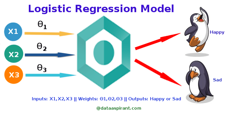
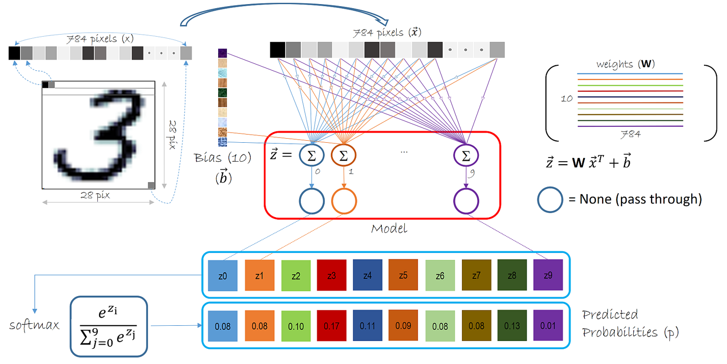
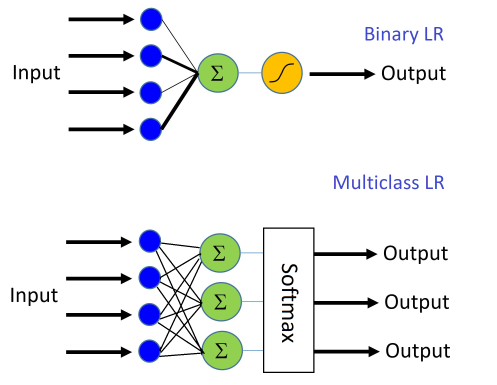
Linear Regression + either Activation or Softmax

Activation: Binary Classification

Softmax: Multi-class Classification

Binary

(image: dataaspirant.com)

Logistic Sigmoid

Converts the output to a value between 0 and 1

• 1 can mean True, Happy, ...
• 0 can mean False, Sad, ...

$$\sigma(x) = \frac{1}{1+exp(-x)}$$

# Credits: https://ilparle.com/2017/04/21/plot-a-simple-sigmoid-function/
import numpy as np
import matplotlib.pyplot as plt

x = np.arange(-8, 8, 0.1)
sigmoid = 1 / (1 + np.exp(-x))

fig, ax = plt.subplots()
ax.plot(x, sigmoid)
ax.set(xlabel = 'x', ylabel = 'sigmoid')
ax.grid()
plt.show()

Multi-Class

(image: CNTK)

Softmax

Softmax:

• Converts multiple outputs to a percentage distribution between 0 and 1
• Percentage distribution: numbers all add up to 1 (100%)
• Outputs: 0.7 happy, 0.2 depressed, 0.1 unknown

Example: [1, 2, 3, 4, 1, 2, 3]

Result: [0.024, 0.064, 0.175, 0.475, 0.024, 0.064, 0.175]

# Credits: https://en.wikipedia.org/wiki/Softmax_function
import numpy as np

z = [1.0, 2.0, 3.0, 4.0, 1.0, 2.0, 3.0]
softmax = lambda x : np.exp(x)/np.sum(np.exp(x))
softmax(z)

(image: CNTK)

Libraries

http://scikit-learn.org/stable/modules/generated/sklearn.linear_model.LogisticRegression.html

# Iris flower dataset
# https://archive.ics.uci.edu/ml/datasets/iris

import sklearn
from sklearn import datasets
from sklearn.model_selection import train_test_split

iris = datasets.load_iris()
X = iris.data
y = iris.target

# Add noisy features to make the problem harder
random_state = np.random.RandomState(0)
n_samples, n_features = X.shape
X = np.c_[X, random_state.randn(n_samples, 200 * n_features)]

X_train, X_test, y_train, y_test = train_test_split(X, y, test_size=0.5, random_state=99)

print('First 5 training data:', X_train[:5])
print('First 5 training labels:', y_train[:5])

from sklearn.linear_model import LogisticRegression

lr = LogisticRegression().fit(X_train, y_train)
y_pred_lr = lr.predict(X_test)

print('Number of mislabeled points out of test set of %d points:' % (X_test.shape[0]))
print('Logistic Regression: %d, Score: %f' % ((y_test != y_pred_lr).sum(), lr.score(X_test, y_test)))

Naive Bayes Classification

(image: shatterline.com)

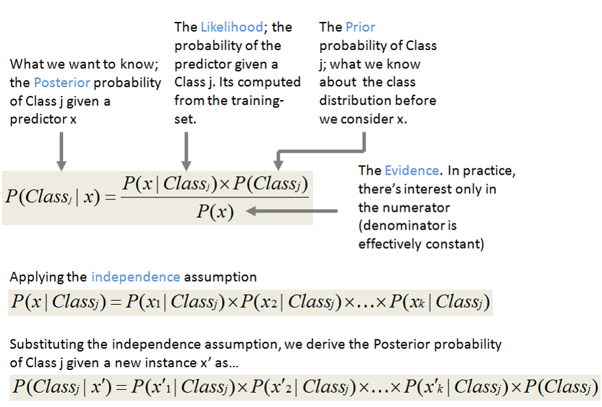
Bayes Theorem

• Inputs: independent features
• Outputs: class probabilities
  • Bayes Theorem computes the conditional probabilities

Libraries

http://scikit-learn.org/stable/modules/naive_bayes.html#naive-bayes

• Gaussian
• Multinomial
• Bernoulli

from sklearn import naive_bayes

# Now that we added noise to our data, we need to scale the features to between [0, 1]
# This is because Naive Bayes cannot handle negative features (throws an error)
from sklearn.preprocessing import MinMaxScaler
min_max_scaler = MinMaxScaler()
min_max_scaler.fit(X_train)
X_train_minmax = min_max_scaler.transform(X_train)
X_test_minmax = min_max_scaler.transform(X_test)

nb_titles = ['Gaussian Naive Bayes', 'Multinomial NB', 'Bernouilli NB']
nb_models = (naive_bayes.GaussianNB(),
             naive_bayes.MultinomialNB(),
             naive_bayes.BernoulliNB())
nb_models = (model.fit(X_train_minmax, y_train) for model in nb_models)

print('Number of mislabeled points out of test set of %d points:' % (X_test.shape[0]))

for model, title in zip(nb_models, nb_titles):
    y_pred = model.predict(X_test_minmax)
    wrong = (y_test != y_pred).sum()
    score = model.score(X_test_minmax, y_test)
    print('%s: %d (score: %.2f)' %(title, wrong, score))

Support Vector Machines

(image: Wikipedia)

Support Vector Machines

• Inputs: features (not necessarily independent)
  • Features should be scaled

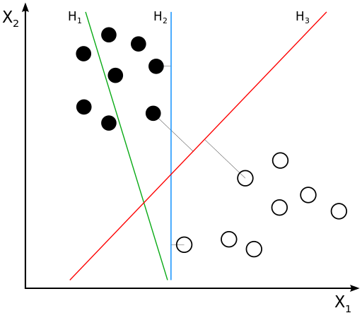
• Output: classes, separated by "hyperplane"

• SVM uses "kernel functions" to compute the similarity between input samples

• Find hyperplane with the maximum margin of separation
  • Why? Better generalization

Libraries

http://scikit-learn.org/stable/modules/generated/sklearn.svm.SVC.html

• Support Vector Classifier
• Different kernel functions to choose from

Scikit-learn has a nifty example that shows how the different kernel functions look like.

To illustrate them, we'll use their code example to train SVM models with only 2 features.

• Why 2 features? Because it's easier to plot in 2-D

# http://scikit-learn.org/stable/auto_examples/svm/plot_iris.html#sphx-glr-auto-examples-svm-plot-iris-py
from sklearn import svm

def make_meshgrid(x, y, h=.02):
    """Create a mesh of points to plot in

    Args:
        x: data to base x-axis meshgrid on
        y: data to base y-axis meshgrid on
        h: stepsize for meshgrid, optional

    Returns:
        xx, yy : ndarray
    """
    x_min, x_max = x.min() - 1, x.max() + 1
    y_min, y_max = y.min() - 1, y.max() + 1
    xx, yy = np.meshgrid(np.arange(x_min, x_max, h),
                         np.arange(y_min, y_max, h))
    return xx, yy

def plot_contours(ax, clf, xx, yy, **params):
    """Plot the decision boundaries for a classifier.

    Args:
        ax: matplotlib axes object
        clf: a classifier
        xx: meshgrid ndarray
        yy: meshgrid ndarray
        params: dictionary of params to pass to contourf, optional
    """
    Z = clf.predict(np.c_[xx.ravel(), yy.ravel()])
    Z = Z.reshape(xx.shape)
    out = ax.contourf(xx, yy, Z, **params)
    return out

fig, sub = plt.subplots(nrows=2, ncols=2, figsize=(15, 10))
plt.subplots_adjust(wspace=0.4, hspace=0.4)

# Take the first two features. We could avoid this by using a two-dim dataset
X_train_svc = X_train[:, :2]

# LinearSVC uses liblinear, SVC uses libsvm
# Both are different implementations of SVM
svm_titles = ['LinearSVC (liblinear)',
              'SVC (linear kernel)',
              'SVC (RBF kernel)',
              'SVC (3-degree polynomial kernel)']

# we create an instance of SVM and fit our data. We do not scale our
# data since we want to plot the support vectors
C = 1.0  # SVM regularization parameter
svm_2D_models = (svm.SVC(kernel='linear', C=C),
          svm.LinearSVC(C=C),
          svm.SVC(kernel='rbf', gamma=0.7, C=C),
          svm.SVC(kernel='poly', degree=3, C=C))
svm_2D_models = (clf.fit(X_train_svc, y_train) for clf in svm_2D_models)

X0, X1 = X_train_svc[:, 0], X_train_svc[:, 1]
xx, yy = make_meshgrid(X0, X1)

for clf, title, ax in zip(svm_2D_models, svm_titles, sub.flatten()):
    plot_contours(ax, clf, xx, yy,
                  cmap=plt.cm.coolwarm, alpha=0.8)
    ax.scatter(X0, X1, c=y_train, cmap=plt.cm.coolwarm, s=20, edgecolors='k')
    ax.set_xlim(xx.min(), xx.max())
    ax.set_ylim(yy.min(), yy.max())
    ax.set_xlabel('Sepal length')
    ax.set_ylabel('Sepal width')
    ax.set_xticks(())
    ax.set_yticks(())
    ax.set_title(title)

plt.show()

Let's compare the performance of SVM with the other Classification models (Logistic Regression, Naive Bayes)

To do that, we retrain the SVM models with the full features.

Exercise - Train and score SVM using different kernels

Train SVM models for the 4 kernel functions.

For each model:

• Scale X_train and X_test using sklearn.preprocessing.StandardScaler.
  • X_train and X_test are multi-dimensional numpy arrays, so you can pass them directly into the scaler without reshaping.
• Print the number of mislabeled points
• Print the score

Use all the features instead of just the first two.

Which model performs the best?

# Your code here

K-nearest Neighbors

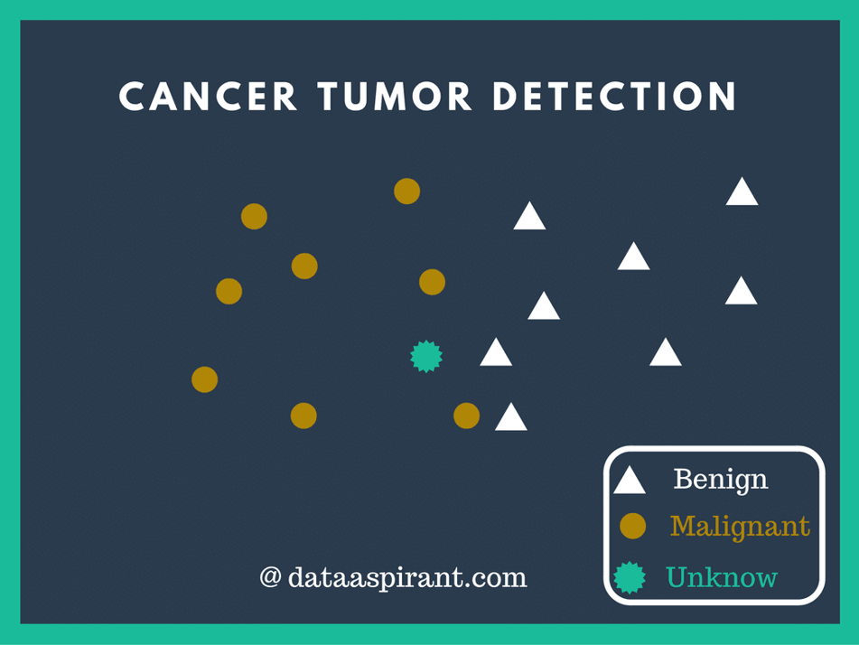
K-nearest neighbors is a multi-purpose algorithm that can be used for multi-class classification.

• Find K closest neighbors to that sample
• Classify by majority vote of the classes of that sample

(image: dataaspirant.com)

Libraries

sklearn.neighbors.KNeighborsClassifier

http://scikit-learn.org/stable/modules/generated/sklearn.neighbors.KNeighborsClassifier.html

from sklearn import neighbors

# K (how many neighbors to consider for the vote)
n_neighbors = [3, 5, 15]

# types of weights
weights = ['uniform', 'distance']

kn_models = []

for k in n_neighbors:
    for weight in weights:
        model = neighbors.KNeighborsClassifier(k, weights=weight)
        model.fit(X_train, y_train)
        y_pred = model.predict(X_test)
        wrong = (y_test != y_pred).sum()
        score = model.score(X_test, y_test)
        print('k = %d, weights = %s: %d (score: %.2f)' %(k, weight, wrong, score))

# http://scikit-learn.org/stable/auto_examples/neighbors/plot_classification.html
import matplotlib.pyplot as plt
from matplotlib.colors import ListedColormap

X_train_plot = X_train[:, :2]
h = .02  # step size in the mesh
n_neighbors = 15

# Create color maps
cmap_light = ListedColormap(['#FFAAAA', '#AAFFAA', '#AAAAFF'])
cmap_bold = ListedColormap(['#FF0000', '#00FF00', '#0000FF'])

for weights in ['uniform', 'distance']:
    clf = neighbors.KNeighborsClassifier(n_neighbors=n_neighbors, weights=weights)
    clf.fit(X_train_plot, y_train)

    # Plot the decision boundary. For that, we will assign a color to each
    # point in the mesh [x_min, x_max]x[y_min, y_max].
    x_min, x_max = X_train_plot[:, 0].min() - 1, X_plot[:, 0].max() + 1
    y_min, y_max = X_train_plot[:, 1].min() - 1, X_plot[:, 1].max() + 1
    xx, yy = np.meshgrid(np.arange(x_min, x_max, h),
                         np.arange(y_min, y_max, h))
    Z = clf.predict(np.c_[xx.ravel(), yy.ravel()])

    # Put the result into a color plot
    Z = Z.reshape(xx.shape)
    plt.figure(figsize=(10, 8))
    plt.pcolormesh(xx, yy, Z, cmap=cmap_light)

    # Plot also the training points
    plt.scatter(X_train_plot[:, 0], X_train_plot[:, 1], c=y_train, cmap=cmap_bold,
                edgecolor='k', s=20)
    plt.xlim(xx.min(), xx.max())
    plt.ylim(yy.min(), yy.max())
    plt.title("3-Class classification (k = %i, weights = '%s')"
              % (n_neighbors, weights))

plt.show()

A Quick Comparison

Criteria	Logistic Regression	Naive Bayes	SVM	K-nearest neighbors
Interpretability	Simple	Very simple (Conditional Probabilities)	Hard to understand parameters	Simple, but need to pick K
Ease of training	Fast to train	Fast to train	Computationally and memory intensive for high dimensional data	Can be expensive for high dimensional data
Requires independent features	Yes, but may still work	Yes, assumes independence	No (don't care)	No (don't care)
Feature value ranges	No requirements, scale if vary too widely	No negative features	Must scale to [-1, 1]	No requirements
Output usefulness	Returns probabilities and categories	Returns probabilities and categories	Returns probabilities and categories	Returns probabilities and categories

Confusion Matrix

Truth/Prediction	Predicted Happy	Predicted Sad
Actually Happy	True positive count	False negative count
Actually Sad	False positive count	True negative count

Example

Truth/Prediction	Predicted Happy	Predicted Sad
Actually Happy	4	3
Actually Sad	2	1

Accuracy

Meaning: what proportion of the samples did the classifier predict correctly?

$$accuracy(y\_true, y\_pred) = \frac{true\_positives + true\_negatives}{total}$$

What's the accuracy in our example?

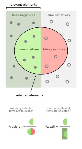
Precision

Meaning: of the samples the classifier predicted TRUE, what proportion did it get correct (i.e. actually true)? The goal is to reduce false positives.

$$precision(y\_true, y\_pred) = \frac{true\_positives}{true\_positives + false\_positives}$$

What's the precision in our example?

Recall (True Positive Rate / Sensitivity)

Meaning: of all the TRUE samples, what proprtion did the classifier predict to be TRUE? (How many of the TRUE predictions did the classifier recall)

$$recall(y\_true, y\_pred) = \frac{true\_positives}{true\_positives + false\_negatives}$$

What's the recall in our example?

Specificity (True Negative Rate)

Meaning: of all the FALSE samples, what proportion did the clasifier predict to be FALSE?

$$specificity(y\_true, y\_pred) = \frac{true\_negatives}{true\_negatives + false\_positives}$$

What's the specificity in our example?

F1 score / F measure

Meaning: a combination of both Precision and Recall in 1 number. This is a harmonic mean of two numbers that uses the standard equation 2AB/(A+B).

$$F(y\_true, y\_pred) = 2 * \frac{precision * recall}{precision + recall}$$

What do they mean?

(image: Wikipedia)

Libraries

http://scikit-learn.org/stable/modules/model_evaluation.html#classification-metrics

• classification_report
• confusion_matrix
• accuracy_score
• f1_score
• ...

from sklearn.metrics import classification_report, confusion_matrix

print('Logistic Regression:')
print(classification_report(y_test, y_pred_lr))

cm = confusion_matrix(y_test, y_pred_lr)
print(cm)

# Colormaps:
# https://matplotlib.org/gallery/color/colormap_reference.html
plt.matshow(cm, cmap='Blues')
plt.colorbar()

iris.target_names # the integer values [0, 1, 2] map to these labels

Exercise - Evaluation Metrics for Naive Bayes and SVM Classifiers

For the Naive Bayes and SVM models we've seen so far:

1. Get the classification metrics.
2. Plot the confusion matrix
3. How would you interpret the results?

# Get the classification metrics
# Your code here

# Plot the confusion matrices for Naive Bayes
# Your code here

# Plot the confusion matrices for SVM
# Your code here

Area under ROC curve

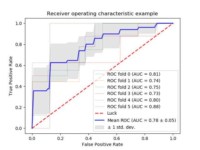
ROC curve: Receiver Operating Characteristic

A plot of True Positive Rate (Recall) vs. False Positive Rate (1-Specificity)

Larger area under ROC curve: better performance

Area under ROC curve

(image: scikit-learn)

Libraries

sklearn.metrics.roc_curve: http://scikit-learn.org/stable/modules/generated/sklearn.metrics.roc_curve.html

sklearn.metrics.auc: http://scikit-learn.org/stable/modules/generated/sklearn.metrics.auc.html

ROC curves and Multi-class Classification

• ROC is typically for binary classification
• To plot ROC for multi-class:
  • Either draw 1 curve per class
  • Or compute average for all the classes

# http://scikit-learn.org/stable/auto_examples/model_selection/plot_roc.html
from sklearn.multiclass import OneVsRestClassifier
from sklearn.metrics import roc_curve, auc
from sklearn.preprocessing import label_binarize

iris = datasets.load_iris()
X = iris.data

# binarize the y labels
y = label_binarize(iris.target, classes=[0, 1, 2])

n_classes = y.shape[1]
print(y)

# Add noisy features to make the problem harder
random_state = np.random.RandomState(0)
n_samples, n_features = X.shape
X = np.c_[X, random_state.randn(n_samples, 200 * n_features)]

# Shuffle and split train/test
X_train, X_test, y_train, y_test = train_test_split(X, y, test_size=.5,
                                                    random_state=42)

classifier = OneVsRestClassifier(LogisticRegression())

y_score = classifier.fit(X_train, y_train).decision_function(X_test)
y_score

# Compute ROC curve and AROC for each class
fpr = dict()
tpr = dict()
roc_auc = dict()
for i in range(n_classes):
    fpr[i], tpr[i], _ = roc_curve(y_test[:, i], y_score[:, i])
    roc_auc[i] = auc(fpr[i], tpr[i])

# Plot the ROC curves
fig, ax = plt.subplots(figsize=(15, 10))

for i in range(n_classes):
    ax.plot(fpr[i], tpr[i], label='ROC curve of class %d (area = %0.2f)' % (i, roc_auc[i]))
ax.legend()