Topics

• Series vs. DataFrames
• Querying, indexing, slicing
• Combining and splitting data
• Handling missing data
• Continuous vs. categorical data

Workshop: Pandas and Data Manipulation

In this workshop, we will use pandas to load, describe, and query datasets.

Cheatsheet

https://s3.amazonaws.com/assets.datacamp.com/blog_assets/PandasPythonForDataScience.pdf

References

1. https://pandas.pydata.org/pandas-docs/stable/
2. Python Data Science Handbook by Jake VanderPlas
3. Python for Data Analysis: Data Wrangling with Pandas, NumPy, and IPython by Wes McKinney
4. https://pandas.pydata.org/pandas-docs/stable/comparison_with_sql.html

Installation

Windows: Start Button -> "Anaconda Prompt"

Ubuntu / MacOS: conda should be in your path

Activate the environment

conda activate mldds01

Pandas should already be installed. If not, install it:

conda install pandas

Tip: You can check the versions installed by calling Python with a script:

python -c "import pandas; print(pandas.__version__)"

SGD to USD Exchange Rate Data

Similar to the NumPy workshop, we'll use the historical SGD to USD exchange rates from data.gov.sg to demonstrate some Pandas concepts.

from IPython.display import IFrame

IFrame('https://data.gov.sg/dataset/exchange-rates-sgd-per-unit-of-usd-average-for-period-annual/resource/f927c39b-3b44-492e-8b54-174e775e0d98/view/43207b9f-1554-4afb-98fe-80dfdd6bb4f6', width=600, height=400)

Download Instructions

You should already have this dataset from the NumPy workshop. If not, here are the instructions:

1. Go to https://data.gov.sg/dataset/exchange-rates-sgd-per-unit-of-usd-average-for-period-annual
2. Click on the Download button
3. Unzip and extract the .csv file. Note the path for use below.

Note: on Windows, you may wish to rename the unzipped folder path to something shorter.

Import the package

import pandas as pd

pd?

Two main data structures

1. Series
2. DataFrame

Series

pandas.Series(data=None, index=None, dtype=None, name=None, copy=False, fastpath=False)

• Similar to 1-d numpy array but with more flexible explicit indexing
• Has two components : index and value for each element
• A bit similar concept as dictionary
• more here..

DataFrame

pandas.DataFrame(data=None, index=None, columns=None, dtype=None, copy=False)

• The primary pandas data structure
• Tabular format similar to excel
• Two-dimensional, potentially heterogeneous tabular data
• structure with labeled axes (rows and columns). Row and columns index
• Can be thought of as a dict-like container for Series objects.
• more here..

Read data from CSV to a Series

You can use pandas.read_csv to read data into:

• A Series, if the data contains only 1 column and you specify the squeeze=True option, or
• A DataFrame, for any number of columns. This is the default behavior because the DataFrame is the most flexible.

more here

# Read data into a series
#
# parse_dates: which column(s) to parse dates
# index_col: which zeroth indexed column to use the index
# infer_datetime_format may speed up the date parsing
sgd_usd_series = pd.read_csv('/tmp/exchange-rates/exchange-rates-sgd-per-unit-of-usd-daily.csv',
                             parse_dates=['date'], index_col=0, infer_datetime_format=True,
                             squeeze=True)

# inspect the first 10 values
sgd_usd_series.head(10)

sgd_usd_series.describe()

# Read data into a data frame
sgd_usd_df = pd.read_csv('/tmp/exchange-rates/exchange-rates-sgd-per-unit-of-usd-daily.csv',
                         parse_dates=['date'], index_col=0, infer_datetime_format=True)

# inspect the first 10 values
sgd_usd_df.head(10)

sgd_usd_df.describe()

# Read data without parsing dates
temp = pd.read_csv('/tmp/exchange-rates/exchange-rates-sgd-per-unit-of-usd-daily.csv',
                   index_col=0)

# inspect the first 10 values
temp.head(10)

# dtype of index is a string
temp.index

# with parse_dates = ['date'], dtype of index is a datetime64
sgd_usd_df.index

# read_csv has many other functions for reading in CSV data
# such as custom parsing functions, or custom delimiters
pd.read_csv?

Get values or indices

Series

• use series.values
• use series.index

DataFrame

• use df.values
• use df.index

Note: these are properties, not function calls with ()

For this dataset:

• Series.values is a 1 dimensional numpy.array

• DataFrame.values is not. It's actually 2 dimensional:

  number of samples (rows) x 1 (column)

This is because DataFrame is a more general data structure that can hold more columns.

sgd_usd_series.values

sgd_usd_df.values

sgd_usd_series.values.shape

sgd_usd_series.values.ndim # rank = 1

sgd_usd_df.values.shape

sgd_usd_df.values.ndim # rank = 2

# Tip: you can flatten the 3993 x 1 numpy array
sgd_usd_df.values.flatten()

The .index is the same whether it is a Series or a DataFrame

sgd_usd_series.index

sgd_usd_df.index

Get the summary

Try these on sgd_usd_series and sgd_usd_df.

df.columns	Describe DataFrame columns
df.info()	Information on a DataFrame
s.count(), df.count()	Number of non-NA values
s.count()	Number of non-NA values

Note: these are from the Cheatsheet. Series supports fewer methods.

Get statistics

Try these on sgd_usd_series and sgd_usd_df.

s.sum(), df.sum()	Sum of values
s.cumsum(), df.cumsum()	Cummulative sum of values
s.min()/s.max(), df.min()/df.max()	Minimum/maximum values
s.idxmin()/series.idxmax(), df.idxmin()/df.idxmax()	Minimum/Maximum index value
s.describe(), df.describe()	Summary statistics
s.mean(), df.mean()	Mean of values
s.median(), df.median()	Median of values

Note: these are from the Cheatsheet

Joins

Let's say we need to also show Singapore Dollar and Renminbi (CNY) exchange rates, but from a different data set.

This dataset is already downloaded for you in the data folder.

# data source: https://www.exchangerates.org.uk
sgd_cny_df = pd.read_csv('data/sgd_cny_rates_daily.csv',
                          parse_dates=True, index_col=0, infer_datetime_format=True)
print('First 5 entries:')
sgd_cny_df.head(5)

sgd_cny_df.info()

sgd_usd_df.info()

sgd_cny_df: DatetimeIndex: 3224 entries, 2018-05-27 to 2009-10-06

sgd_usd_df: DatetimeIndex: 3993 entries, 1988-01-08 to 2015-10-19

• have different date ranges
• one is in decreasing time order, the other is increasing time order

Pandas DataFrames make it easy to join these datasets together based on index.

You can do this without looping over the data, using DataFrame.join()

more info..

sgd_usd_df.join?

# Default join is an `left` join, where the index of the left series (`sgd_usd_df`) is preserved.

sgd_usd_cny = sgd_usd_df.join(sgd_cny_df)
sgd_usd_cny

We can remove the NaN entries using dropna()

sgd_usd_cny = sgd_usd_cny.dropna()
sgd_usd_cny

The result is a DataFrame with entries where both exchange rates are present.

Entries where either SGD-USD or SGD-CNY are missing are excluded.

Note that even though the index for the series are in different order, join will still work because it matches the individual index values

When in doubt, visualize

Let's visualize what we just did by plotting the dataframes.

You should have already installed matplotlib. If not, do this:

conda install matplotlib

# Find the names of the columns
sgd_usd_cny.columns

import matplotlib.pyplot as plt

fig, (ax1, ax2) = plt.subplots(nrows=2, ncols=1, figsize=(20,15),
                              sharex=True) # common x-axis for all subplots

ax1.set_title('Original series')
ax1.plot(sgd_usd_df, label='SGD/USD')
ax1.plot(sgd_cny_df, label='SGD/CNY')
ax1.legend(loc='upper center', shadow=True, fontsize='x-large')

ax2.set_title('After join() and dropna()')
ax2.plot(sgd_usd_cny['exchange_rate_usd'], label='SGD/USD')
ax2.plot(sgd_usd_cny['Singapore Dollar to Chinese Yuan'], label='SGD/CNY')
ax2.legend(loc='upper center', shadow=True, fontsize='x-large')

plt.show()

sgd_cny_usd = sgd_cny_df.join(sgd_usd_df).dropna()
fig, (ax1, ax2) = plt.subplots(nrows=2, ncols=1, figsize=(20,15),
                              sharex=True) # common x-axis for all subplots

ax1.set_title('Original series')
ax1.plot(sgd_usd_df, label='SGD/USD')
ax1.plot(sgd_cny_df, label='SGD/CNY')
ax1.legend(loc='upper center', shadow=True, fontsize='x-large')

ax2.set_title('After join() and dropna()')
ax2.plot(sgd_cny_usd['exchange_rate_usd'], label='SGD/USD')
ax2.plot(sgd_cny_usd['Singapore Dollar to Chinese Yuan'], label='SGD/CNY')
ax2.legend(loc='upper center', shadow=True, fontsize='x-large')

plt.show()

Pandas, like SQL

If you have worked with SQL or databases before, the DataFrame.join() is conceptually the same as SQL.

Here's a guide that compares Pandas with SQL.

This SQL:

SELECT *
FROM tips
WHERE time = 'Dinner' AND tip > 5.00;

Becomes this in pandas:

tips[(tips['time'] == 'Dinner') & (tips['tip'] > 5.00)]

We'll do an example with queries to demonstrate how you can think of Pandas as conceptually equivalent to SQL.

Exercise: Querying a DataFrame

Let's say you want to query a DataFrame using something equivalent to this SQL syntax:

SELECT *
FROM sgd_usd_cny
WHERE date >= '2012-01-01' AND date < '2013-01-01';

What will you use in Pandas?

# Use pandas to find all exchange rates from 2012, for the sgd_usd_cny DataFrame
#
# Refer to https://pandas.pydata.org/pandas-docs/stable/comparison_with_sql.html
#
# Hint 1: use pd.to_datetime
# start = pd.to_datetime('2012-01-01')
# end = pd.to_datetime('2013-01-01')
#
# Hint 2: use sgd_usd_cny.index to compare against the date time
#
# Hint 3: add parenthesis for the boolean conditions

Indexing and Slicing: iloc, loc

iloc	Select by position
loc	Select by label
iat	Get scalar value by position (fast iloc)
at	Get scalar value by label (fast loc)

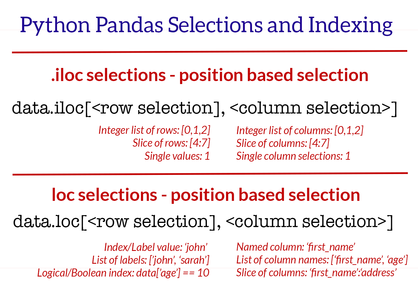(image: shanelynn.ie)

loc, at

sgd_usd_cny.loc[:4] # error (because index is time, not integer) 

# use a DateTimeIndex for row selector
sgd_usd_cny.loc[pd.to_datetime('2009-10-08'), :]

# use a column selector
sgd_usd_cny.loc[pd.to_datetime('2009-10-08'), 'exchange_rate_usd']

# fast single-value access using .at
sgd_usd_cny.at[pd.to_datetime('2009-10-08'), 'exchange_rate_usd']

iloc, iat

sgd_usd_cny.iloc[1, :] # select by row position

sgd_usd_cny.iloc[1]['exchange_rate_usd'] # select by row position, column name

sgd_usd_cny.iat[1, 0] # select by row position, column position

sgd_usd_cny.iloc[:4, :] # select by row slice

Combining with boolean conditions

# logical / boolean row index
sgd_usd_cny.loc[sgd_usd_cny.exchange_rate_usd < 1.21, :]

# more selectors
sgd_usd_cny.loc[sgd_usd_cny.exchange_rate_usd > 1.425]['Singapore Dollar to Chinese Yuan']

# iloc does not support boolean indexing, because it is NOT label-based

sgd_usd_cny.iloc[sgd_usd_cny.exchange_rate_usd < 1.21, :] # error

Adding and removing rows / columns

s.drop(), df.drop()	Drop row (axis=0)
s.drop('col', axis=1), df.drop('col', axis=1)	Drop column (axis=1)
pd.concat([s1, s2], axis=0), pd.concat([df1, df2], axis=0)	Concatenate rows (axis=0)
pd.concat([s1, s2], axis=1), pd.concat([df1, df2], axis=1)	Concatenate columns (axis=1)

pd.concat?

pd.DataFrame.drop?

# Append a few rows of empty data
index = pd.date_range(start='2015-10-20', end='2015-10-22')

new_df = pd.DataFrame(index=index,
                      columns=sgd_usd_cny.columns)
result = pd.concat([sgd_usd_cny, new_df], axis=0) # axis=0 for rows
result.tail(10)

# Drop the rows
index = pd.date_range(start='2015-10-20', end='2015-10-22')

result.drop(index, inplace=True)
result.tail(10)

Exercises: add and remove columns

1. Add a new column called 'SGD to Euro' with empty values
2. Drop the column you just added

# Add a new column called 'SGD to Euro', with empty values
#
# Hint 1: use index=sgd_usd_cny.index
# Hint 2: what value should axis be in pd.concat?
#

# Drop the column you just added
# 
# Hint: use inplace=True so that the change is performed in place
# Hint: what value should axis be?
#

Missing data

We saw how to add columns and rows without any data. Now we'll explore how to deal with the missing data.

Here are some ways:

dropna	Drop missing values
fillna(new_value)	Fill missing values with new_value
interpolate()	Use linear interpolation

We've already seen how dropna() works.

pd.DataFrame.dropna?

pd.DataFrame.fillna?

pd.DataFrame.interpolate?

index=pd.date_range(start='2015-10-20', end='2015-10-22')

new_df = pd.DataFrame(index=index,
                      columns=sgd_usd_cny.columns)
result = pd.concat([sgd_usd_cny, new_df], axis=0)
result.tail(10)

# Dropping the NaN values
result.dropna().tail(5)

# Filling the NaN values with a meaningful value, such as the median
median = result.median()
result.fillna(median).tail(5)

# Using linear interpolation
result.interpolate().tail(5)

Categorical Data

The previous dataset shows how to use pandas for datasets with continous variables (the exchange rate).

Let's see another dataset that demonstrates how to use pandas for categorical variables (such as classes of things).

We'll use the Annual Motor Vehicle Population by Vehicle Type dataset from data.gov.sg.

Reference: https://pandas.pydata.org/pandas-docs/stable/visualization.html

Download Instructions

1. Go to https://data.gov.sg/dataset/annual-motor-vehicle-population-by-vehicle-type
2. Click on the Download button
3. Unzip and extract the .csv file. Note the path for use below.

df = pd.read_csv('/tmp/motor-vehicles/annual-motor-vehicle-population-by-vehicle-type.csv',
                 parse_dates=['year'], index_col=0, infer_datetime_format=True)
df

Grouping and aggregating categories

Since this series has multiple entries for the same date, we can group rows together using group_by.

For example, to find the total number of vehicles per year:

df.groupby(df.index)['number'].sum()

We can also plot the total number of vehicles per year:

ax = df.groupby(df.index)['number'].sum().plot(marker='o')
ax.set(ylabel='Vehicle Population',
       xlabel='Year',
       title='Annual Vehicle Population')

Processing per category

# get the unique classes
df.category.unique()

# get just the dataFrame for a category
buses = df[df.category =='Buses']
buses.head(5)

# count of each category
for name in df.category.unique():
    print(name, df.loc[df.category == name, "category"].count())

# pick a year (2009) and plot the distributions across types
df_2009 = df[df.index == pd.to_datetime('2009')]
df_2009

# Create a series with the type as the index, and the numbers as values
s_2009_type = df_2009.number
s_2009_type.index = df_2009.type
s_2009_type

# plot the bar chart
s_2009_type.plot.bar()

# Let's ignore private cars because they outweigh everything else
s_2009_type[s_2009_type.index != "Private cars"].plot.bar()

Pivot Table

Pandas supports creating a pivot table, similar to what is available from Excel.

This is useful when we would like to group categories by year, and then display them in stacked bar plots, with year on the x-axis.

pandas.pivot_table()

bar plots

Why pivot table?

The original dataset has each category as a separate entry in the category column.

year	category	type	number
2005-01-01	Cars & Station-wagons	Private cars	401638
2005-01-01	Cars & Station-wagons	Company cars	14926

For the bar plot, we need each category as a separate column. The entry under each category will be the number of vehicles for that year.

Something like:

year	Buses	Cars & Station-wagons	Goods & Other Vehicles	...
2005-01-01	2640	438194	128193	...
2006-01-01	...	...	...	...

# Original dataset, filtered by year 2005 as an illustration
df[df.index == pd.to_datetime('2005')]

Create pivot table that is:

• indexed by year
• using category as the columns
• numbers as values

Each category has multiple entries (one for each type), so we also need to specify this:

• aggregate function to sum up the numbers for that category

import numpy as np
pv_year_category = pd.pivot_table(df, index="year", columns="category",
                                  values="number", aggfunc=np.sum)

pv_year_category

Hmm, there are some NaN values.

On closer examination, the culprit is 2017, where "and" replaced "&" in the category name.

We will need to fix those entries so that the name matches.

Question

Can you explain why can't we just use dropna(axis=1) to drop columns with NaN?

# Show the problematic dataframes (2017)
df_2017 = df.loc[pd.to_datetime('2017'), :]
df_2017

Exercise

Fix the category names for year = 2017 by replacing "and" with "&".

Avoid looping on individual rows.

For a given category, you can:

1. Use the syntax df.loc[row_indexer, col_indexer] to get a view for each incorrect category
2. Assign the correct value to that view

Note on why we use DataFrame.loc:

Using df.loc with assignment will avoid this SettingWithCopyWarning, because loc returns a view, not a copy of the DataFrame:

Traceback (most recent call last)
     ...
SettingWithCopyWarning:
     A value is trying to be set on a copy of a slice from a DataFrame.
     Try using .loc[row_index,col_indexer] = value instead

# Your code needs to fix these categories:
#
#     Incorrect                   Correct
#     ---------------------------------------------------
#     Cars and Station-wagons     Cars & Station-wagons
#     Goods and Other Vehicles    Goods & Other Vehicles
#     Motorcycles & Scooters      Motorcycles
#     ----------------------------------------------------
#

# Your code here













# Let's generate the pivot_table again, the NaNs should now go away
pv_year_category = pd.pivot_table(df, index="year", columns="category",
                                  values="number", aggfunc=np.sum)

pv_year_category

Let's plot the bar chart.

We are doing a bit more matplotlib stuff here to make the bar chart readable.

fig, ax = plt.subplots(figsize=(10,8))

pv_year_category.plot(kind='bar', stacked=True, ax=ax)
ax.set(title='Annual Motor Vehicle Population by Category',
       ylabel='Vehicle Population',
       xlabel='Year')
ax.legend(loc='upper left')

# Due to: https://github.com/pandas-dev/pandas/issues/1918
# Can't just do: ax.xaxis.set_major_formatter(mdates.FormatStrFormatter('%Y'))
ax.xaxis.set_major_formatter(plt.FixedFormatter(pv_year_category.index.to_series().dt.strftime("%Y")))

fig.tight_layout()
plt.show()