(image: numpy.org)

Topics

• Vectors, Matrices, and Tensors
• Indexing, Slicing, Reshaping, Transposing
• Sorting, Broadcasting

Workshop: NumPy and Data Representation

In this workshop, we will explore numpy data structures, indexing and slicing, and transformations.

Cheatsheet

https://s3.amazonaws.com/assets.datacamp.com/blog_assets/Numpy_Python_Cheat_Sheet.pdf

More cheatsheets: https://www.datacamp.com/community/data-science-cheatsheets?page=3

References

1. https://docs.scipy.org/doc/numpy-dev/user/basics.types.html
2. Python Data Science Handbook by Jake VanderPlas
3. Python for Data Analysis: Data Wrangling with Pandas, NumPy, and IPython by Wes McKinney

Installation

Windows: Start Button -> "Anaconda Prompt"

Ubuntu / MacOS: conda should be in your path

Activate the environment

conda activate mldds01

Install NumPy and Pandas

(mldds01) conda install numpy pandas

Tip: You can check the versions installed by calling Python with a script:

python -c "import numpy; print(numpy.__version__)"

SGD to USD Exchange Rate Data

Instead of constructing sample arrays, we'll be using real data to play with numpy concepts.

We'll use some data from data.gov.sg.

from IPython.display import IFrame

IFrame('https://data.gov.sg/dataset/exchange-rates-sgd-per-unit-of-usd-average-for-period-annual/resource/f927c39b-3b44-492e-8b54-174e775e0d98/view/43207b9f-1554-4afb-98fe-80dfdd6bb4f6', width=600, height=400)

Download Instructions

1. Go to https://data.gov.sg/dataset/exchange-rates-sgd-per-unit-of-usd-average-for-period-annual
2. Click on the Download button
3. Unzip and extract the .csv file. Note the path for use below.

Note: on Windows, you may wish to rename the unzipped folder path to something shorter.

Read the CSV

We'll be using a little bit of Pandas to read the CSV files.

Pandas will be covered in more detail in the next Workshop.

import pandas as pd

# we are using some pandas tricks to parse dates automagically
sgd_usd = pd.read_csv('D:/tmp/exchange-rates/exchange-rates-sgd-per-unit-of-usd-daily.csv',
                     parse_dates=True, index_col=0, infer_datetime_format=True,
                     squeeze=True)

# get the numpy array
sgd_usd_values = sgd_usd.values

sgd_usd_values

Where did the dates go? They are part of the pandas Series:

# inspect the first 5 entries of the Series
sgd_usd.head(5)

Import numpy

import numpy as np

# show help
np?

Basic Data Structures

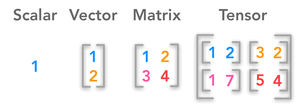
(image: https://hadrienj.github.io/posts/Deep-Learning-Book-Series-2.1-Scalars-Vectors-Matrices-and-Tensors/)

Scalar

A scalar is a single value.

It is a tensor of rank 0. (0 dimension)

# get the first value of the array
print('First value:', sgd_usd_values[0])

# get the last value of the array
print('Last value:', sgd_usd_values[-1])

# to get the rank of a scalar, we need to wrap it in a numpy.array
v = sgd_usd_values[-1]
print('Rank:', np.array(v).ndim)

Vector

A vector is a list of values.

It is a tensor of rank 1. (1 dimension)

sgd_usd_values.shape

sgd_usd_values.ndim

sgd_usd_values.dtype

Matrix

A matrix is a 2-dimensional array of values.

It is a tensor of rank 2.

There are many ways to create a matrix. For this dataset, we can stack the arrays to create a matrix.

matrix = np.array((sgd_usd_values, sgd_usd_values))
matrix

matrix.shape

matrix.ndim

Stacking is not the same as concatenation.

Here's an example of concatenation. What do you think is the difference?

concat_array = np.concatenate((sgd_usd_values, sgd_usd_values))
concat_array

Here's a hint:

concat_array.shape

We can keep stacking vectors to make matrices.

matrix_stacked = np.vstack((matrix, matrix))
matrix_stacked

matrix_stacked.shape

matrix_stacked.ndim

We can also try horizontal stacking, which is the same as concatenating.

matrix_hstacked = np.hstack((matrix, matrix))
matrix_hstacked

matrix_hstacked.shape

matrix_stacked.ndim

Tensor (rank $\geq$ 3)

A tensor is a data structure of values that has more than 3 dimensions.

An image is an example of a tensor.

To load an image, we can use pillow:

(mldds01) conda install pillow

We'll also install the requests library to download images from the web:

(mldds01) conda install requests

from PIL import Image
import requests

url = 'https://upload.wikimedia.org/wikipedia/commons/8/81/Singapore_Merlion_BCT.jpg'

image = Image.open(requests.get(url, stream=True).raw)
tensor = np.array(image)
tensor

tensor.shape # rows, columns, channels

tensor.ndim

Data Structure Manipulation

Now we'll look at indexing, slicing, and subsetting.

The concepts apply to vectors, matrices, and tensors.

# Array documentation
from numpy import doc

# Array types and conversions, scalars
doc.basics?

# Array indexing and slicing
doc.indexing?

Indexing

tensor[0]

matrix[0]

sgd_usd_values[0]

tensor[0][1]

matrix[0][1]

sgd_usd_values[0][1] # error. Why?

Negative indexing

tensor[-1][-1][-1]  # last row, column, channel scalar

matrix[0][-2] # first row, 2nd last column scalar

sgd_usd_values[-len(sgd_usd_values)] # first scalar

Boolean indexing

# returns all values > 1.4
sgd_usd_values[sgd_usd_values > 1.4]

# boolean indexing always returns a vector
matrix[matrix < 1.4]

Subsetting (fancy indexing)

A[index, ...]

sgd_usd_values[[1, 2, -1]]

tensor[0]

tensor[0, 0]

tensor[0, 1]

tensor[0, 2]

row = [0, 0, 0]
col = [0, 1, 2]
tensor[row, col]

tensor[:, :, 0].shape # everything for the 1st channel

Slicing

data[start : stop : stepsize]

sgd_usd_values[0: 9: 1]

matrix[0][0: 9: 1]

tensor[0: 500: 1, :].shape # first 500 rows

Let's use matplotlib to show what the slicing does.

(mldds01) conda install matplotlib

from matplotlib import pyplot as plt
plt.imshow(tensor[0: 500: 1, :]) # first 500 rows, all columns
plt.axis('off')
plt.show()

Exercises

Write the code to show rightmost 500 vertical lines of the original image.

# Your code below
# 1. Get the slice for the last 500 columns.
# 2. Use plt.imshow to display the slice.

Slices are views, not copies

Changes to a slice will change values in the original data structure.

# Make a copy of the original tensor using numpy.copy
tensor_save = np.copy(tensor)

top_500_rows = tensor[0: 500: 1, :]

# Change the channel to zero for the first 500 rows
top_500_rows[:,:,-1] = 0

# Compare the two side-by-side
fig, (ax1, ax2) = plt.subplots(nrows=1, ncols=2, figsize=(20,10))

ax1.imshow(tensor)
ax1.axis('off')
ax1.set_title('modified')

ax2.imshow(tensor_save)
ax2.axis('off')
ax2.set_title('saved copy')
plt.show()

Transposing

tensor.T

tensor.T.shape # channels, cols, rows

Sorting

sgd_usd_values

# sort, ascending
np.sort(sgd_usd_values)

# sort, descending
np.sort(sgd_usd_values)[::-1] # ::-1 means iterate backwards

sgd_usd_values_save = np.copy(sgd_usd_values) # save a copy (for comparison only)

# sort, descending, in-place
sgd_usd_values[::-1].sort()
sgd_usd_values # array has been sorted in place

# compare with original values
fig, (ax1, ax2) = plt.subplots(nrows=1, ncols=2, figsize=(20,10))

ax1.plot(sgd_usd_values)
ax1.set_title('sorted')

ax2.plot(sgd_usd_values_save)
ax2.set_title('copy')

plt.show()

# sort by row
np.sort(tensor, axis=0)

# sort by column
np.sort(tensor, axis=1)

fig, (ax1, ax2, ax3, ax4) = plt.subplots(nrows=1, ncols=4,
                                         figsize=(20,10))

tensor = tensor_save # restore

ax1.imshow(tensor)
ax1.axis('off')
ax1.set_title('unsorted')

ax2.imshow(np.sort(tensor, axis=1))
ax2.axis('off')
ax2.set_title('sorted by column')

ax3.imshow(np.sort(tensor, axis=0))
ax3.axis('off')
ax3.set_title('sorted by row')

ax4.imshow(np.sort(tensor, axis=2))
ax4.axis('off')
ax4.set_title('sorted by channel')

plt.show()

Computations

sgd_usd_values = sgd_usd_values_save # revert

# Rather than doing subplots, we'll overlay the plots on the same axis (ax)
fig, ax = plt.subplots(figsize=(20,15))

ax.plot(sgd_usd_values, label='original')

mean = np.mean(sgd_usd_values)
ax.plot(sgd_usd_values - mean, label='subtract mean (%.2f)' % mean)

ax.plot(sgd_usd_values * 2, label='2x')

ax.plot(1 / sgd_usd_values, label='inverse')

ax.plot(np.log(sgd_usd_values), label='log')

ax.plot(np.exp(sgd_usd_values), label='exponential')

legend = ax.legend(loc='upper right', shadow=True, fontsize='x-large')
plt.show()