My first machine learning model

(image: flickr)

Topics

• The end-to-end process
• A simple linear regression model
• Data Preparation
• Training
• Evaluation Metrics

Workshop

In this workshop, we will walk through creating and training a simple machine learning model from scratch.

Through out the course, we'll be repeating the tasks in this process for different machine learning algorithms.

Data Science Process

(image: szilard)

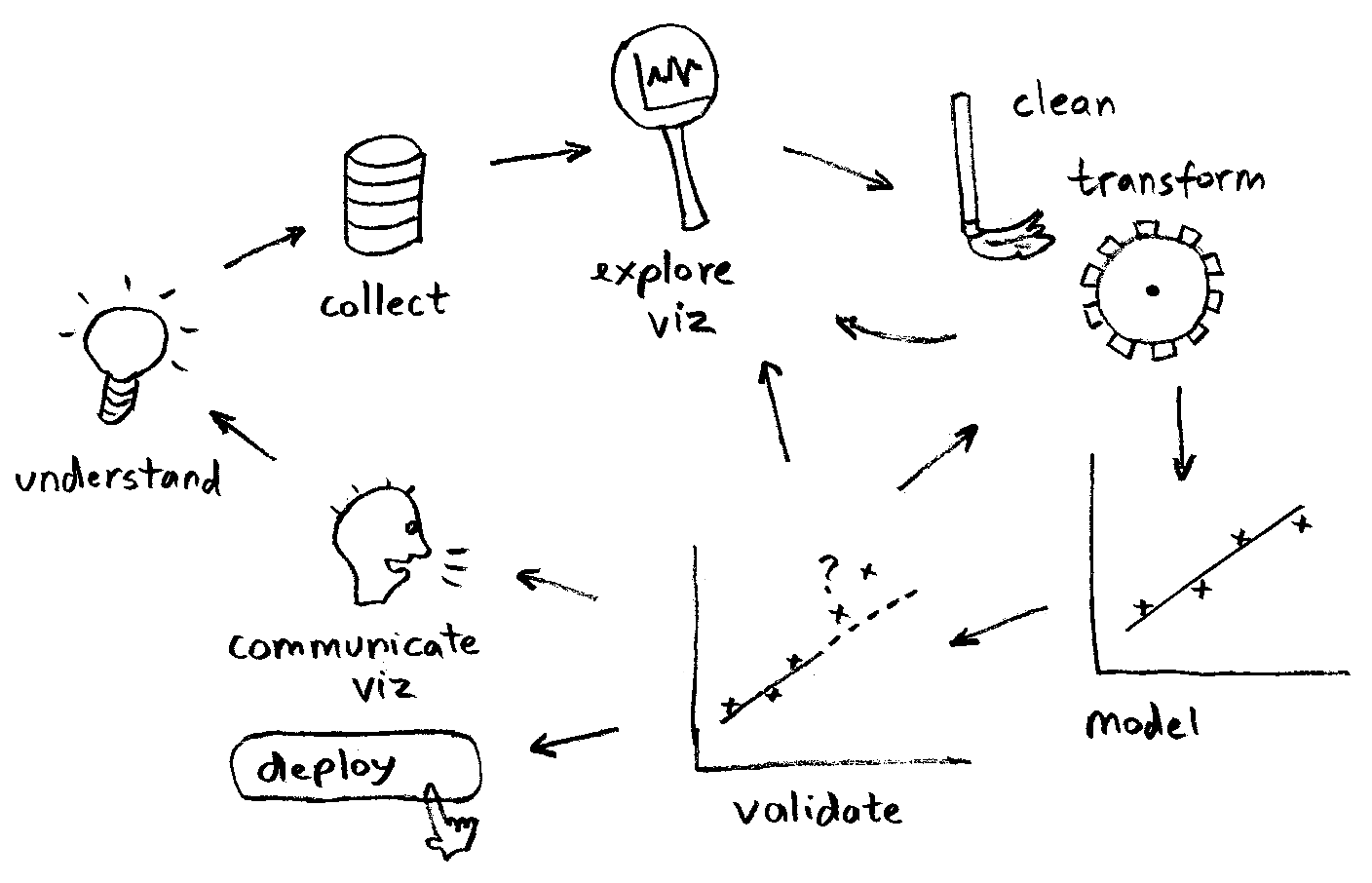
What we will cover today

1. Data transformation and cleaning
2. Feature selection
3. Model creation and training
4. Model validation
5. Undestanding results and iterating

Prediction Task

For our first machine learning problem, we will try to predict Singapore's Foreign Reserves based on Gross Domestic Product (GDP).

Datasets

1. Gross Domestic Product at Current Prices, Annual: https://data.gov.sg/dataset/income-components-of-gross-domestic-product-at-current-prices-annual
2. Total Foreign Reserves: https://data.gov.sg/dataset/total-foreign-reserves

• Download both datasets
• Note their paths for use later, when we call pandas.read_csv.

Installation: scikit-learn

Install scikit-learn, a machine learning library that we'll use in this and subsequent modules.

conda install scikit-learn

More information about scikit-learn: http://scikit-learn.org

import numpy as np
import pandas as pd
import matplotlib.pyplot as plt
import sklearn

1. Data Transformation and Cleaning

The first step is to inspect the data. We are looking for a relationship between GDP and Foreign Reserves.

First, we have the Annual Gross Domestic Product, which is our independent variable.

Let's notate it as x, so the corresponding DataFrame will be df_x.

df_x = pd.read_csv('D:/tmp/income-components-of-gross-domestic-product-at-current-prices-annual/gross-domestic-product-at-current-market-prices-annual.csv',
                parse_dates=['year'], index_col=0)
df_x.head()

Next, we have the Annual Total Foreign Reserves, which is our dependent variable (we think it is dependent on X).

Let's notate is as y, so the corresponding DataFrame will be df_y.

df_y = pd.read_csv('D:/tmp/total-foreign-reserves/total-foreign-reserves-annual.csv',
                parse_dates=['year'], index_col=0)
df_y.head()

Looks like df_x has a different date range than df_y. Let's print the ranges to confirm:

print('Time range of df_x:', df_x.index.values.min(), df_x.index.values.max())
print('Time range of df_y:', df_y.index.values.min(), df_y.index.values.max())

Joining the datasets

Since we have two datasets, let's join them into a single DataFrame.

We will do:

• a left join of df_y onto df_x, and
• drop any NaN values

This will also take care of the different date ranges.

df = df_x.join(df_y).dropna()
df

Scatter plot to inspect possible relationships

Let's also plot the relationship between X and Y.

Between 2 or 3 variables, a scatter plot is useful to see if the (x, y) points lie on some sort of line or curve.

fig, ax = plt.subplots(figsize=(20, 10))
df.plot(kind='scatter', x='value', y='total_foreign_reserve_sgd', ax=ax)

ax.set(xlabel='Annual GDP S$ million',
       ylabel='Annual Total Foreign Reserves S$ million')
ax.grid()

for index, row in df.iterrows():
    ax.annotate(index.strftime('%Y'), (row['value'], row['total_foreign_reserve_sgd']))

Play around with other columns as well, to explore the data further and observe other relationships.

fig, ax = plt.subplots(figsize=(20, 10))
df.plot(kind='scatter', x='value', y='imf_reserve_position', ax=ax) # less linear

ax.set(xlabel='Annual GDP S$ million', ylabel='IMF Reserve Position S$ million')
ax.grid()

for index, row in df.iterrows():
    ax.annotate(index.strftime('%Y'), (row['value'], row['imf_reserve_position']))

2. Feature selection

For this simple task, feature selection is straightforward.

No further transformation is needed because:

• The data is already in numerical format, and we've dropped missing values.
• There's only one feature, so there no need to normalize the features by scaling or re-centering them.

Inputs

Feature	Description	Column name	Transformation before model input?
$x_1$	Annual GDP S$ million	value	None

Outputs

Output	Description	Truth column	Transformation from model output?
$\hat{y}$	Predicted Annual Foreign Reserves S\$ million	$y$ = total_foreign_reserve_sgd	None

Here's our resulting dataset after feature selection:

data = {'x1': df.value.values, 'y': df.total_foreign_reserve_sgd.values}
df_dataset = pd.DataFrame(data=data)
df_dataset.head()

3. Model creation and training

In this section, we'll train a simple single-variable Linear Regression model.

Linear Regression

Textbook definition:

• Linear regression takes a vector x ($x \in \Re$) as input, and predicts the value of a scalar y ($y \in \Re$) as output.
• Let $\hat{y}$ be the value that the model predicts, then:

$$\hat{y} = w^Tx,$$

where

• $w^Tx$ is known as the linear function of the input
• $w \in \Re$ are the parameters or weights of that linear function

(Reference: Deep Learning - Goodfellow, Bengio, Courville, MIT press, 2016)

Application to our problem

This table summarizes how Linear Regression will be applied to our machine learning problem.

Variable	What it is	What are its values	How is it used
$x_1$	Scalar feature	Annual GDP	Used as training inputs
$w_1$	Scalar weight	Learned by model	Used for computing $\hat{y}$
$\hat{y}$	Scalar prediction	Result of $w^Tx$	Used for training output
$y$	Scalar truth or target	Annual Foreign Reserves	Used for minimizing training error (cost)

Note that we use subscripts here, $x_1$ and $w_1$ because we only have a scalar input value.

Derivation of Linear Function

You may recall that a linear function has a y-intercept term, $b$:

$$\hat{y} = w_1x_1 + b$$

This is sometimes also called the "bias" (because it "shifts" the output by a constant value)

If we rewrite the above equation as:

$$\hat{y} = w_0x_0 + w_1x_1$$

where $x_0 = 1$, and $w_0 = b$

Then, it becomes the following vector-vector product:

$$\hat{y} = \left(\begin{array}{c c} w_0 & w_1 \end{array} \right) \left(\begin{array}{c} x_0 \\ x_1 \end{array} \right)$$

Which is our "textbook" linear function:

$$\hat{y} = w^Tx$$

Example Linear Functions

Let's plot some examples of linear functions.

# inputs
x1 = np.arange(-5, 5, 1)
x0 = np.ones(x1.shape)
x = np.vstack([x0, x1])

# weights
w1 = np.array([1, -4, 8]) # slope
w0 = np.array([-6, 0, 6]) # y-intercept
w = np.vstack([w0, w1])

# linear function
y_hat = np.dot(w.T, x)

fig, ax = plt.subplots(figsize=(10, 5))
for i in range(0, y_hat.shape[0]):
    ax.plot(x1, y_hat[i], label='{}x + {}'.format(w1[i], w0[i]))
ax.grid()
ax.legend()
ax.set(title='Single-variable linear functions', xlabel='x', ylabel='y_hat')
plt.show()

Training Linear Regression

Let's train our Linear Regression model in Python using scikit-learn.

Train/Test split

To train a model, it is good practice to split your data into two sets:

• training set
• test set

This allows the model to avoid "overfitting", which is when the model is "too specific" to the data we give it.

• The danger of overfitting is that the model can only work well with the data we've used to train it.
• To avoid this, we usually "hold back" some of the data for "independent testing". This becomes the test set.

The above is the layman's explanation. We'll cover overfitting in more formal detail in the next module.

hold_back_percent = 20
sample_size = len(df_dataset)
test_sample_size = int(np.rint(hold_back_percent * sample_size / 100))

print('number of data samples', sample_size)
print('training test split', hold_back_percent)
print('number of samples reserved for testing', test_sample_size)

Shuffle the dataset

Before doing the train/test split, we'll also shuffle the data so we can make the training and testing more "fair" (or closer to real life usage of the model).

df_dataset_shuffled = df_dataset.sample(frac=1).reset_index()

df_dataset_shuffled.head()

df_train = df_dataset_shuffled.iloc[0:-test_sample_size]
df_test = df_dataset_shuffled.iloc[-test_sample_size:-1]

df_train.head()

df_test.head()

Create and train model

We'll use sklearn.linear_model.LinearRegression to fit our model.

from sklearn.linear_model import LinearRegression

model = LinearRegression()

# LinearRegression is designed generically to work with multiple features,
# and expects x to be a 2D array.
x1_train = df_train.x1.values.reshape(-1, 1) # add 1 extra dimension

%time model.fit(x1_train, df_train.y)

print('Coefficient (w1)', model.coef_)
print('Intercept (w0)', model.intercept_)

4. Model Validation

Now that we've trained our model, the next step is to evaluate how well training went.

Steps:

1. Get predictions, $\hat{y}$, using LinearRegression.predict()
2. Compute the mean-squared error and r2 score of the predictions against the truth $y$.
   • A smaller mean-squared error is better
   • A variance score of 1 means a perfect prediction

from sklearn.metrics import mean_squared_error, r2_score

# LinearRegression is designed generically to work with multiple features,
# and expects x to be a 2D array.
x1_test = df_test.x1.values.reshape(-1, 1)
y_test = df_test.y.values

y_hat = model.predict(x1_test)

print('Truth:', y_test)
print('Predictions:', y_hat)

mean_squared_error(y_test, y_hat)

r2_score(y_test, y_hat)

Huh?

Hmm, the mean-squared error is really high. What's going on?

Since the R2 score is actually quite good, we consult the formula of mean-squared error:

The numerical values are in tens and hundreds of thousands. A relatively "small" difference of hundreds can be magnified to thousands, summed across the number of test samples.

Let's try mean_squared_log_error instead.

from sklearn.metrics import mean_squared_log_error

mean_squared_log_error(y_test, y_hat)

Much better...

Plot predictions vs. truth

Finally, let's visualize the predictions against the truth.

fig, ax = plt.subplots(figsize=(10, 5))

y_hat_train = model.predict(x1_train)

ax.plot(y_hat_train, x1_train, label='prediction (test)')
ax.plot(y_hat, x1_test, label='prediction (train)')

ax.scatter(y_test, x1_test, marker='x', label='truth (test)')
ax.scatter(df_train.y.values, x1_train, marker='x', label='truth (train)')

ax.set(xlabel='Annual GDP S$ million',
       ylabel='Annual Total Foreign Reserves S$ million')
ax.legend()
ax.grid()

What do we get in the end?

In the (involved) process of training a machine learning model, it can be easy to forget what we actually get in the end.

Summary

1. What: we've trained a linear regression model based on historical annual GDP and foreign reserves data, to try to find a relationship between the two.

2. Metrics: MLSE of 0.022, R2-score of 0.999

3. This model can be deployed to predict the Total Foreign Reserves, given the Annual GDP.

Deployment use case

Note that the actual use case is not that realistic, because Foreign Reserves are affected by other factor as well, such as policy decisions.

This brings up another interesting point. Whereas machine learning can find correlation parameters, it won't tell you if the correlation actually makes sense.

# Imagine you are the future Finance Minister,
# here's how the model might be used in deployment scenarios

gdp = np.array([200000, -200000, 0, 50000000])
predicted_foreign_reserves = model.predict(gdp.reshape(-1, 1))

for i in range(len(gdp)):
    print('S$%d million GDP => Foreign Reserves S$%.2f million'
         %(gdp[i], predicted_foreign_reserves[i]))

Reading List

Material	Read it for	URL
Deep Learning Basics, Chapter 5, Pages 105-107	Linear Regression Theory	http://www.deeplearningbook.org/contents/ml.html
Ordinary Least Squares Linear Regression	Programming Example	http://scikit-learn.org/stable/modules/linear_model.html#ordinary-least-squares

from IPython.display import YouTubeVideo

YouTubeVideo('VlpFaak0ZKs')